Suppose you are going to count the average working hours of employees in the company based on different months. If a worksheet including working hours on different dates and months is prepared for you, do you know how can we calculate the average of working hours based on months?

In this article, through explaining the example below, we will introduce you though creating a formula with AVERAGEIFS function and EOMONTH function inside to return average working hours for different months. You can get the basic knowledge and usage of these two functions in this article.

EXAMPLE

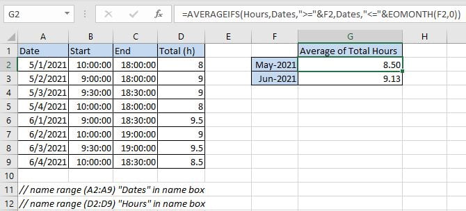
We can see that “Start” time and “End” time are recorded clearly for different dates from above table. Total hours are calculated correctly as “Start” minus “End”, the unit is hour. In “Date” column, dates belong to two months “May” and “June”. To calculate average of total hours, we need to calculate average separately for the two months respectively.

For F2 (May-2021) and F3 (Jun-2021), in fact we input date 05/01/2021 into F2 and 06/01/2021 into F3, and set custom format “mmm-yyyy” for the two cells, then they are displayed as “May-2021” and “Jun-2021”. Only in this way they can be processed properly in the following operation.

We want to create only one formula that can be used for returning average working hours based on different months properly, in case of range reference auto adjusted when copying the formula, we use named ranges “Dates” and “Hours” to represent range references (A2:A9) and (D2:D9) in this instance.

In this article, to approach our goal, we will apply AVERAGEIFS function with EOMONTH function inside.

ANALYSIS

a. To calculate average, first we can think about average related functions like AVERAGE, AVERAGEIF, AVERAGEIFS etc.

b. As dates in “Date” belong to two months “May” and “June”, to calculate the average of total hours for one of them, we need to filter dates from “Date” column and make sure they belong to month “May” properly (or “June”); if dates meet our condition, total hours in “Total” will be kept and come to average calculation.

c. To filter date by condition “belong to May”, dates are required to meet below conditions:

1) Date >= 05/01/2021. // date should be greater than or equal to the first date in May.

2) Date <= 05/31/2021. // date should be less than or equal to the last date in May.

As we are going to calculate total hours from “Total” column based on filtered dates, and there are two conditions to filter date from given named range “Date”, so we can select AVERAGEIFS function to calculate average with multiple conditions to solve our problem in this instance.

d. To return the last date of a month, we can apply Excel EOMONTH function. Depends on the given date in F2, it can return the last date of the same month.

Above all, we can create formula =AVERAGEIFS(Hours,Dates,”>=”&F2,Dates,”<=”&EOMONTH(F2,0)) to solve this problem.

FORMULA

Input formula

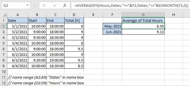
=AVERAGEIFS(Hours,Dates,">="&F2,Dates,"<="&EOMONTH(F2,0))

into G2 and press Enter, verify that 8.50 is returned and shown in G2 properly. As (8+9+8+9)/4=8.5. The return value is correct.

Notice: actually, the returned value may be a number with more than two decimal places (based on your settings), you can click “Decrease Decimal” in “Number” section under Home tab to shorten decimal places and keep only two.

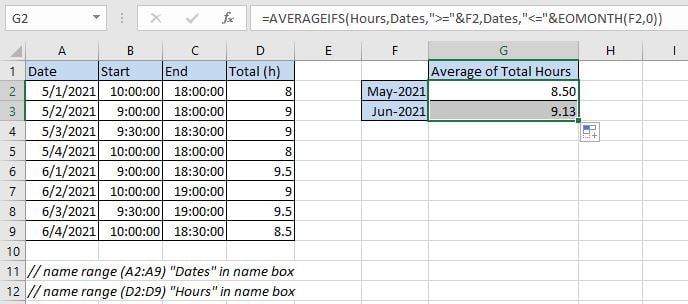
Drag the handle down to copy formula to G4, verify that 9.13 is returned properly.

FUNCTION INTRODUCTION

a. AVERGAEIFS function can be seen as AVERAGE+IFS. It returns the average of a set of numbers in range based on one or more given conditions or criteria.

Syntax:

=AVERAGEIFS (average_range, criteria_range1, criteria1, [criteria_range2], [criteria2], ...)

 Example.

b. EOMONTH function returns the last date of month based on the given date.

Syntax:

 =EOMONTH(start_date, months)

 Comment: Argument months is a serial number; n months represents n months before or after the input start date. For example, if A1 is 05/20/2021, we enter =EOMONTH(A2, 1), it returns 06/30/2021 (set cell in proper date format). If we enter =EOMONTH(A2, -1) (negative value in months), it returns 04/30/2021. If we enter =EOMONTH(A2, 0), it returns 05/31/2021.

Example.

EXPLANATION

=AVERAGEIFS(Hours,Dates,">="&F2,Dates,"<="&EOMONTH(F2,0))

// average range is named range “Hours” (D2:D9)

// criteria range1 and criteria range2 are the same named range “Dates” (A2:A9)

// criteria 1 is “>=”&F2 (F2: date 5/1/2021)

// criteria 2 is “<=”&EOMONTH(F2,0)

a. The first criteria is “>=”&F2, it is combined with logical operator “greater than or equal to” (“>=”) and cell reference F2, they are concentrated by “&”. Value in F2 is “5/1/2021”, but when running the formula, it is converted to number “44317” which represents the date 5/1/2021.

b. The second criteria is “<=”&EOMONTH(F2,0). EOMONTH function returns the last day of one month which is decided by the entered date. For F2 date is 5/1/2021, the second argument months is 0, so EOMONTH() returns the last day of May, it is 05/31/2021. Date 05/31/2021 is displayed as 44347 if change format from date to general format.

c. Then filter dates from “Dates” by the two conditions.

d. After filtering dates by providing conditions, then calculate average of hours refer to the filtered dates.

e. After running above steps, formula returns average value “8.5” properly. In fact, you can select formula in formula bar, and press F9, you can find the formula returns 8.5 directly.

Video: Average of Working Hours by Formula

This Excel video tutorial, we’ll explore the use of the AVERAGEIFS and EOMONTH functions to efficiently compute monthly averages based on your dataset.

Related Functions

• Excel AVERAGE function
  The Excel AVERAGE function returns the average of the numbers that you provided.The syntax of the AVERAGE function is as below:=AVERAGE (number1,[number2],…)….
• Excel AVERAGEIF function
  The Excel AVERAGEAIF function returns the average of all numbers in a range of cells that meet a given criteria.The syntax of the AVERAGEIF function is as below:= AVERAGEIF (range, criteria, [average_range])….
• Excel AVERAGEIFS function
  The Excel AVERAGEAIFS function returns the average of all numbers in a range of cells that meet multiple criteria.The syntax of the AVERAGEIFS function is as below:= AVERAGEIFS (average_range, criteria_range1, criteria1, [criteria_range2, criteria2],…)….