Financial choices play a critical role in the development and execution of corporate strategies and plans. In daily life, we also face a slew of financial choices. For instance, suppose you’re applying for a loan to purchase a new automobile. It will undoubtedly be beneficial to discover the actual interest rate you will be required to pay your bank. Excel has the excel RATE function for such circumstances, which is specifically intended to calculate the interest rate for a certain term.

Excel rate function

RATE is an Excel financial function that calculates the interest rate on an annuity over a specified time. The function calculates iteratively and may return zero or more solutions.

Excel 365, Excel 2019, Excel 2016, Excel 2013, Excel 2010, and Excel 2007 all provide this feature.

The following is the syntax:

=RATE(nper, pmt, pv, [fv], [type], [guess])

Where:

• Nper (needed) – the total number of payment periods, which may include years, months, and quarters.
• Pmt (mandatory) – the set monthly payment amount that cannot be adjusted throughout the annuity’s life. It typically includes principle and interest but excludes taxes.
• Pv (needed) – the present value of the loan or investment, i.e. its current worth.
• Fv (optional) – the future value, that is, the cash balance you desire to have after the previous payment. If omitted, the default value is 0.
• Type (optional) – specifies the manner in which payments are made:
• 0 or omitted (default) – payment is due at the end of the term
• Guess (optional) – your best guess for the rate. If left blank, it defaults to 10%.

Note:

• The RATE function performs trial and error calculations. If it does not reach a solution after 20 iterations, it returns a #NUM! error.
• By default, interest is computed on a per-payment basis. However, as seen in this example, you can get an annuity solve for interest rate by multiplying.
• While the RATE syntax specifies pv as a mandatory parameter, it may actually be removed if the fv argument is included. Typically, this syntax is used to calculate the interest rate on a savings account.
• In most circumstances, the guess parameter may be deleted since it serves just as a beginning value for an iterative method.
• When computing RATE for various periods, ensure that the values for nper and guess are constant. For instance, if you’re making yearly payments on a two-year loan with an annual interest rate of 4%, use 2 for nper and 4% for estimate.
• If you’re making monthly payments on the same loan, use 2*12 for the nper and 4% /12 for the estimate.

RATE formula Examples

In this example, we’ll look at the easiest way to create a RATE formula in Excel for the purpose of calculating interest rates.

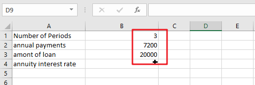
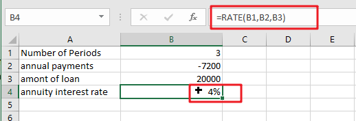
Assume you borrowed $20,000 and are required to repay it in full over the following three years. You intend to pay three annual payments of $7200 each. How much will interest cost on a yearly basis?

Please note that the yearly payment (pmt) is specified as a negative figure since it is an outgoing cash payment.

Assuming that the payment will be paid at the end of each year, we may omit or change the parameter to the default value. Also deleted are the two optional parameters and guess.

As a consequence, we get the following straightforward formula:

=RATE(B1,B2,B3)

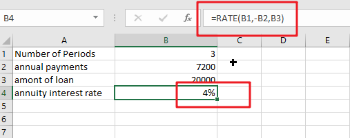
If the payment must be recorded as a positive integer, include the negative sign exactly before the pmt parameter in the formula:

=RATE(B1,-B2,B3)

Now that you’re familiar with the fundamentals of utilizing RATE in Excel, let’s look at a few particular use scenarios.

Determine a Loan’s Monthly Interest Rate

Given that the majority of installment loans are repaid monthly, it may be advantageous to know the monthly interest rate, correct? This is accomplished by providing an adequate number of payment periods to the RATE function.

Assume the loan is to be repaid in monthly installments over a two-year period. We multiply two years by twelve months to get the total amount of payments (2*12=24).

The remaining parameters are listed below:

• Nper (number of periods) in A1: 24
• Pmt (monthly payment) in A2: -1000
• Pv(load amount) in A3: 20000

Assuming the payment is due at the end of each month, the monthly interest rate may be calculated using the well-known formula:

=RATE(B1,B2,B3)

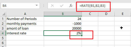
Calculate the interest rate on a monthly basis in Excel

If your source data contains the number of years required to repay the loan, you may do the multiplication inside the nper argument:

=RATE(B1*12,B2,B3)

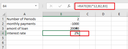
Calculate annuity for Interest rate on Monthly Payments

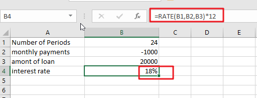
Continuing our example, how do you calculate the yearly interest rate on monthly payments? Simply multiply the RATE value by the number of periods in a year, which in our instance is twelve:

=RATE(B1,B2,B3)*12

Calculate Quarterly Interest Rate

Assume the loan is to be repaid in quarterly installments over a two-year period. We multiply two years by 4 quarters to get the total amount of payments (2*4=8).

To begin, the entire number of periods is converted to quarterly:

Nper: 2 (years) multiplied by 4 (quarters per year) equals 8.

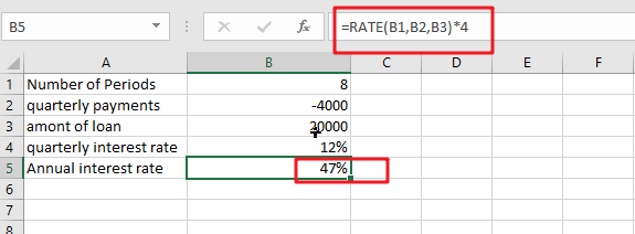
Then, compute the quarterly interest rate in cell B4 using the RATE function:

=RATE(B1,B2,B3)

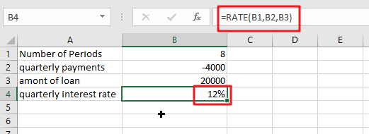
If you want to get the yearly interest rate based on quarterly interest rate, you still need to multiply the quarterly interest rate by four, using the following formula:

=RATE(B1,B2,B3)*4

Related Functions

• Excel RATE function
  The Excel RATE function returns the interest rate per payment period of an annuity.The syntax of the RATE function is as below:=RATE(nper, pmt,pv,[fv],[type],[guess])….