Calculating the difference between two times might be a valuable statistic for subsequent computations or averages, whether you’re producing a time sheet for staff or recording personal exercises. While Excel has a plethora of complex functions, including date and time functions, calculating time elapsed is not always obvious. If you’re calculating time differences of less than 24 hours, you may use the simple HOUR function; otherwise, you’ll need to create a new formula that accounts for longer time disparities. In this post we’ll calculate number of hours between two times.

Table of Contents
How to use Excel to determine time difference (elapsed time)
To begin, let’s look at how to easily compute elapsed time in Excel, that is, how to determine the difference between a starting and ending time. Additionally, as is often the case, there are several formulas for doing time computations. Which one to choose is determined on the size of your dataset and the precise nature of the outcome you are attempting to attain. Therefore, let us go through each approach one by one.
When There Are Less Than 24 Hours
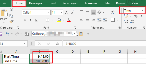
Step 1: In the first cell, enter a time in the “hh:mm:ss” format and, if required, add “AM” or “PM” Enter the same information a second time in another cell using the same format. Excel will default to “AM” if you do not input “PM,” or “AM.”

Step 2: Select both cells and then click the formatting window in the “Home” tab’s Number group. The formatting window’s title may read “General” or something else entirely. To format the cells as time, choose “Time“

Step 3:To begin, click an empty cell. Enter an equal sign followed by the unquoted phrase “hour” Substitute an open parenthesis for the preceding. After entering the later time, click the cell with the “-” symbol. Select the first cell that corresponds to the earlier time you entered. Replace the opening parenthesis with a closing parenthesis. Subtract the first time from the second time by pressing “Enter” For instance:
=HOUR(B2-B1)

When 24 Hours or More
Step 1: In one cell, enter the date and time in the “mm/dd/yyy hh:mm:ss” format; in another cell, enter the date and time in the “mm/dd/yyy hh:mm:ss” format. If required, substitute “AM” or “PM” Separate the date, time, and AM or PM with spaces. For instance: 2022/5/10 9:48:00.
Step 2: Select both cells and then click the formatting window in the “Home” tab’s Number group. The formatting window’s title may read “General” or something else entirely. To open the Format Cells window, click “More Number Formats” Pick “Time” from the Category list on the left, and then navigate through the Type window’s choices to select a date and time format. Select “OK.”
Step 3: To begin, click an empty cell. Enter a “=” symbol followed by the unquoted word “INT“. Two open parentheses are required. Select the cell that contains the more recent time you entered, followed by a “–” symbol. Select the first cell that corresponds to the earlier time you entered. Replace the opening parenthesis with a closing parenthesis. Without quotations, type “*24” and add the last parenthesis. “Enter.” the key. For instance:
=INT((E8-D8)*24)

Related Functions
- Excel HOUR Function
The Excel HOUR function returns the hour of a time value. Or returns an integer value that represent the hour component of a given time. The syntax of the HOUR function is as below:=HOUR (serial_number) … - Excel INT function
The Excel INT function returns the integer portion of a given number. And it will rounds a given number down to the nearest integer.The syntax of the INT function is as below:= INT (number)…