This post will discuss that how to calculate the rate of return for the share of stock in Excel. And to calculate the return for a share of stock, you need to know the starting price, ending price and dividends paid and the duration for which the stock was held.

Calculate Stock Return

You can try to calculate the rate of return by manually, or you use an Excel formula to achieve the result. The best way to calculate your rate of return is to use the EXCEL XIRR function, and this function is a financial function in Excel.

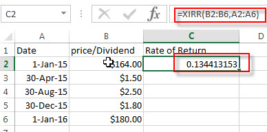
For example, you bought stock “IBM” in 2015, 100 shares for $164 each. And IBM pays dividends quarterly. And the ending price is $180.  And the below is table of dividends, starting price and ending price:

Date	price/Dividend
1-Jan-15	-$164.00
30-Apr-15	$1.50
30-Aug-15	$2.50
30-Dec-15	$1.80
1-Jan-16	$180.00

 

So you can use the below formula to calculate the rate of return for your stock:

=XIRR(B2:B6,A2:A6)

#1 type the above formula in the formula box of cell C2, press enter key. You will get the rate of return of the stock you bought.

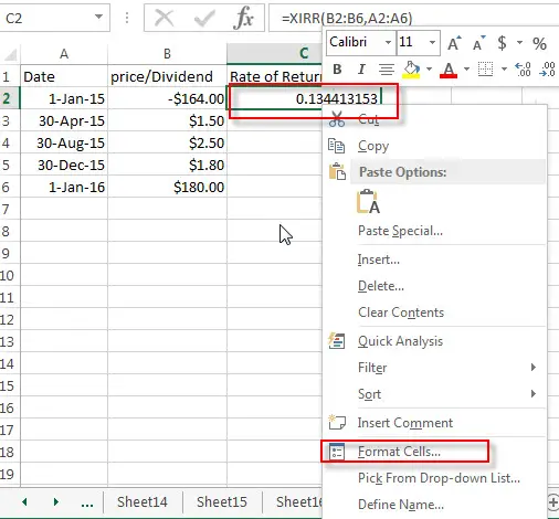
#2 select the cell that contain rate of return (C2), then right-click on it, select Format Cell…  from the drop-down list.

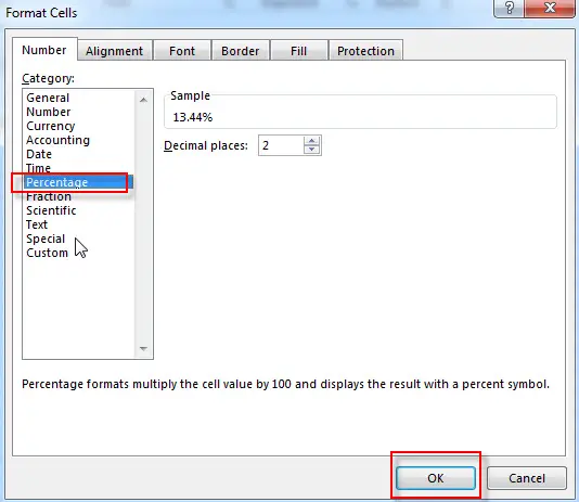
#3 click Percentage under Category section. Click OK button.

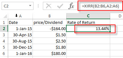
#4 now you can see that the rate of return for your stock is shown as a percentage.

---

Related Functions

• Excel XIRR Function
  The Excel XIRR function returns the internal rate of return for a series of cash flows that is not necessarily periodic.The syntax of the XIRR function is as below:= XIRR (values, dates, [guess])…