In our daily life, most of us will invest or take a loan, so we need to master some simple financial functions to calculate the period needed for loans or investments. If you work as an accountant, you need to master some basic Excel financial functions even more.

In fact, Excel provides many basic financial functions (such as IRR, FV, PMT, etc.). By applying these functions, we can make a simple estimate of interest rate, period, payment, etc.

Today we will introduce an Excel financial function NPER. The function name consists of Number + Period. It is a function often used by accountants. In addition to the basic introduction of the function, we will also provide some examples to illustrate the usage of the function.

NPER FUNCTION

 Excel NPER function is a financial function, based on a fixed interest rate and equal payments, used to calculate the number of periods of a loan or investment.

Syntax:

=NPER(rate,pmt,pv,[fv],[type])

 Arguments:

• rate – it is the interest rate for each period, which is a fixed value
• pmt – it is the amount payable for each period and remains constant throughout the annuity period. Typically, payment includes principal and interest, but excludes other fees and taxes.
• pv – present value. This is the sum of the amounts already accounted for from the beginning of the calculation of the investment, or the cumulative sum of the current values of future payments, also known as the principal.
• fv – future value [optional]. The cash balance after the last payment, if it is omitted, is assumed to have a value of zero, i.e., the future value of a loan is zero.
• type – 0 or 1 to specify whether the payment for each period is at the beginning or at the end of the period. Optional.

NPER FUNCTION EXAMPLES

Example1: Calculate the number of repayment periods for the loan

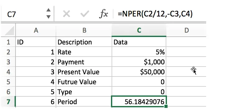
To repay a loan of 50,000 with an annual interest rate of 5% and a monthly repayment of 1,000 (at the end of each month), calculate the number of months required to repay the loan.

In this example, the formula is:

=NPER(C2/12,-C3,C4)

 Rate:

C2/12 (5%/12). Rate in C2 is annual interest rate. Since we want to know the number of periods (months) to repay the loan, we use C2/12 to get the monthly interest rate.

 PMT:

-C3. The equal payment is $1000. Because it is used to pay the loan, it is a cash outflow, so it has a negative value. So for the argument payment, it has a value of “-C3”.

 PV:

C4, present value is $50000. That means we will pay for a loan of $50000.

FV:

The future value of the loan is 0.

Type:

Type is 0. At the end of period.

In this example, the result is 56.18, so it takes 57 months to repay the loan.

Example2: Calculate the number of installments

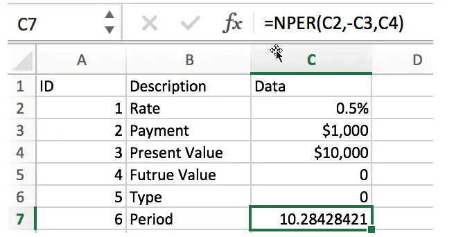
 Suppose an item is purchased at a cost of 10,000, and the monthly payment of 1,000 is made at the end of each month, and the monthly compounding rate is 0.5%, calculate the number of months of repayment.

In this example, the formula is:

=NPER(C2,-C3,C4)

 This example is similar to the previous one. The difference is that this is a monthly interest rate, so you don’t have to divide it by 12 months.

Example3: Calculate the cumulative investment period

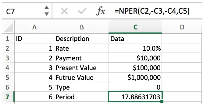
 Suppose the annual rate of return on investment is 10%, now you have invested $100000, add $10000 every year, calculate the number of years to reach 1 million.

In this example, the formula is:

=NPER(C2,-C3,-C4,C5)

 In this example, we are calculating the number of years it would take to reach $1 million with a 10% annual return, so the period is also “years”. Since payments and present value are paid for investments, they are cash outflows, so they are negative in the formula. The future value is out expected value $1 million.

Related Functions

• Excel NPER Function
  The Excel NPER function returns the number of periods for an investment or loan based on periodic payment amount and a constant interest rate.The NPER function is a build-in function in Microsoft Excel and it is categorized as a Financial Function.…