If you are looking for the simplest approach to categorize the text with keywords, then look no further because you have just landed on the right blog post where you will get to know a formula and its usage to get the work done in a matter of seconds.
So, without further ado, let us begin.
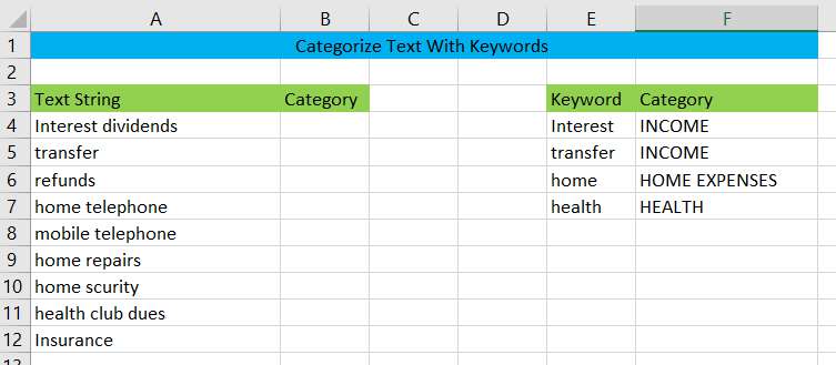
Table of Contents
General Formula
In order to categorize text strings based on some keywords, you can use the following nested formula based on the INDEX function in combination with the SEARCH and MATCH functions.
=INDEX(category,MATCH(TRUE,ISNUMBER(SEARCH(keywords, text_string)),0))
Syntax Explanations
In order to apply this formula to complete your task, you must be familiar with its syntax.
- category – This is the name range $F$4:$F$9.
- Keywords – this is the name range $E$4:$E$9
- INDEX – This function will assist in returning the value at a certain position in a range or array. More information on the INDEX function may be found here.
- ISNUMBER – The ISNUMBER function returns TRUE if a cell contains a number and FALSE otherwise.
- MATCH – It aids in determining the location of a lookup value inside a row, column, or table. More information on the MATCH function may be found here.
- Parenthesis () – This symbol is used to organize the elements.
- SEARCH – The Excel SEARCH function finds the character between two text strings and provides the number of the first text string’s beginning position from the first character of the second text string.
- Text – This is the value from the input table.
- The comma symbol (,)– It is a separator that may be used to separate a list of values.
- TRUE – The TRUE function will assist in returning TRUE if the specified criteria are TRUE or vice versa.
Summary
You may use the SEARCH function, together with INDEX and MATCH, to categorize text using keywords with a “contains” match.
If you need to categorize the text in cell A4, then you can enter the following formula in cell B4.
=INDEX(category,MATCH(TRUE,ISNUMBER(SEARCH(keywords,A4)),0))
where keywords are the named range $E$4:$E$9 and categories is the named range $F$4:$F$9.
This is an array formula, so after you type the above formula, you need to press control + shift + enter to make the above formula as an array formula.
Explanation
This is a typical INDEX/MATCH lookup function , so let’s see how this nested formula works.
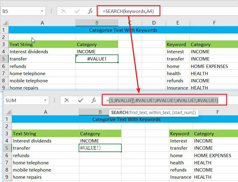
=SEARCH(keywords,A4)
This formula will compare all the keywords in the keyword range with the string in cell A4 and return the first matching position. For example, the keyword “interest” is at position 1 in the string “interest dividends“, but there is no match in the string “transfer“, so it returns #VALUE!.
Since the keywords Name range is an array type, the formula also returns an array with the following values.
{1;#VALUE!;#VALUE!;#VALUE!;#VALUE!;#VALUE!}
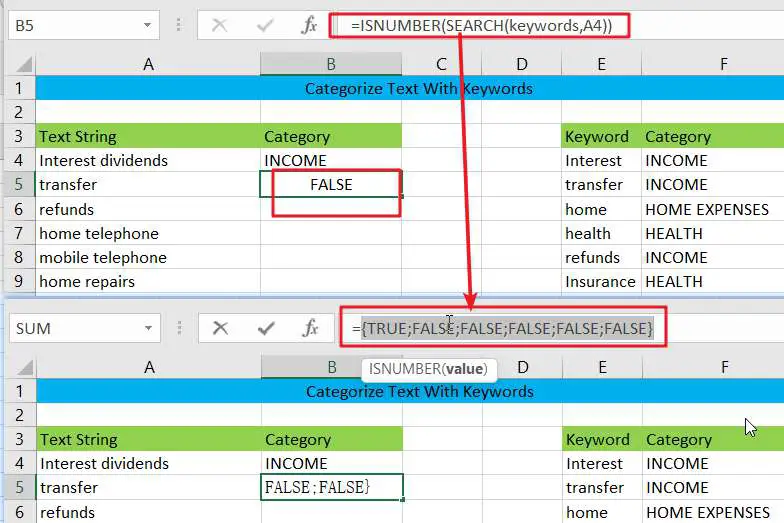
=ISNUMBER(SEARCH(keywords,A4))
In order to have a more usable format for the above return value, you need to convert the #VALUE! error message to a more understandable TRUE/ALSE using the ISNUMBER function. if the return value is #VALUE!, then FALSE is returned, otherwise TRUE is returned.
{TRUE;FALSE;FALSE;FALSE;FALSE;FALSE}
=INDEX(category,MATCH(TRUE,{TRUE;FALSE;FALSE;FALSE;FALSE;FALSE},0))
The above array values are used as arguments to the Index_match formula with a lookup value of TRUE. the MATCH function will return the location of the first TRUE value, and the returned location will be used as an incoming argument to the INDEX function, which returns the category value of the specified location to INDEX.
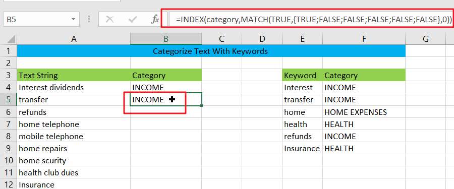
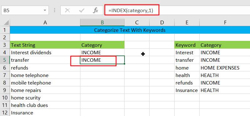
As you can see from the above figure, the INDEX formula needs to return the first value in the category range.
=INDEX(category,1)
Related Functions
- Excel INDEX function
The Excel INDEX function returns a value from a table based on the index (row number and column number)The INDEX function is a build-in function in Microsoft Excel and it is categorized as a Lookup and Reference Function.The syntax of the INDEX function is as below:= INDEX (array, row_num,[column_num])… - Excel ISNUMBER function
The Excel ISNUMBER function returns TRUE if the value in a cell is a numeric value, otherwise it will return FALSE.The syntax of the ISNUMBER function is as below:= ISNUMBER (value)… - Excel SEARCH function
The Excel SEARCH function returns the number of the starting location of a substring in a text string.The syntax of the SEARCH function is as below:= SEARCH (find_text, within_text,[start_num])… - Excel MATCH function
The Excel MATCH function search a value in an array and returns the position of that item.The MATCH function is a build-in function in Microsoft Excel and it is categorized as a Lookup and Reference Function.The syntax of the MATCH function is as below:= MATCH (lookup_value, lookup_array, [match_type])….