This post will guide you how to compare the adjacent cells in the different columns using Conditional Formatting Icon Sets in Excel. How do I compare cells in the adjacent rows using Conditional Formatting Icon Sets in Excel. How to compare Columns or rows using Conditional Formatting Icon Sets to show increase or decrease status in your current worksheet. How to use the conditional formatting feature to show trend arrows when comparing the adjacent columns or rows.

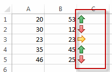
Assuming that you have a list of data A1:B5, and you want to compare cells in Column A with Column B, if the value in Cells in Column B is greater than the value of cells in Column A, then showing an up arrow Icon in the Column C; If the value of cells in Column B is equal to the value in Column A, then showing an right arrow icon in column C; If the value of cells in Column B is less than the value in Column A, then showing an down arrow icon in Column C. How to achieve it.

1. Comparing Columns Using Conditional Formatting Icon Sets

To compare the adjacent columns using conditional formatting icon sets in excel, you need to do the following steps:

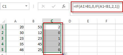
#1 type this formula into the formula box of the first cell in column C, and drag the AutoFill Handler over other cells to apply this formula.

=IF(A1>B1,0,IF(A1<B1,2,1))

This formula will compare the adjacent cells in Column A and B.

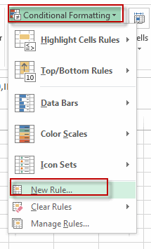
#2 go to HOME tab, Click Conditional Formatting command under Styles group. and select New Rule from the popup menu list. The New Formatting Rule dialog box will appear.

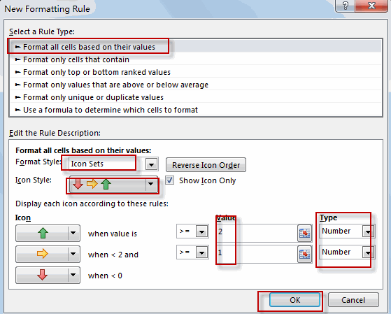
#3 click Format all cells based on their values option from the Select a Rule Type list box. and select Icon Sets value from the drop-down list box of Format Style. Select 3 Arrows icon from the drop-down list of Icon Style. Check Show Icon Only option, and then type the value 2 when the Icon is up arrow icon. and type the value 1 when icon is right icon. Click Ok button.

#4 Let’s see the result.

2. Video: Comparing Columns Using Conditional Formatting Icon Sets

This Excel video tutorial, where we delve into the skill of comparing columns using Conditional Formatting Icon Sets.

https://youtu.be/mLPMN9VQ_5o

3. Related Functions

• Excel IF function
  The Excel IF function perform a logical test to return one value if the condition is TRUE and return another value if the condition is FALSE. The IF function is a build-in function in Microsoft Excel and it is categorized as a Logical Function.The syntax of the IF function is as below:= IF (condition, [true_value], [false_value])….