This post will guide you how to apply conditional formatting for alternate row color based on groups in your worksheet in Excel. How do I alter row color by groups using conditioanl formatting in Excel 2013/2016/2019.

1. Alternating Rows Color by Groups

Assuming that you have a list of data in range A1:B5, in which contain text values, and you want to alter rows background color by groups, you can apply conditional formatting with a formula based on the ISODD function. Just do the following steps:Step1: you need to add a helper column and add a conditional format rule that references the values in the helper column. select cell C1, and enter the number 1.

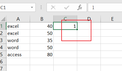
Step2: type the following formula into Cell C2 .

=IF(A2=A1,C1,C1+1)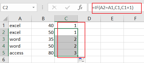

Note: this example will group rows by column A. If you want to group rows by other columns, just replace Cell A2 and A1 with other cells in this formula.

Step3: Copy the formula in Cell C2 to the remaining cells in the range C3:C5.

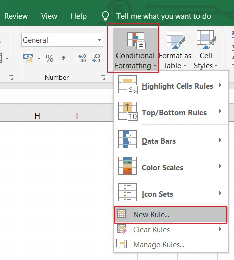
Step4:  select your data range A1:C5, go to HOME tab, click Conditional Formatting command under Styles group, Click New Rule from the drop down menu list. And the New Formatting Rule dialog will open.

Step5: click Use a formula to determine which cells to format option in the New Formatting Rule dialog box, type the following formula in the Format values where this formulas is true text box.

=ISODD($C1)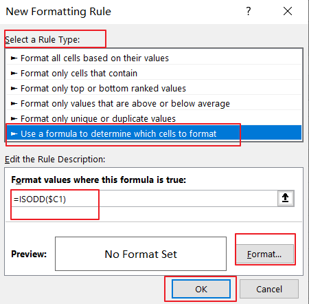

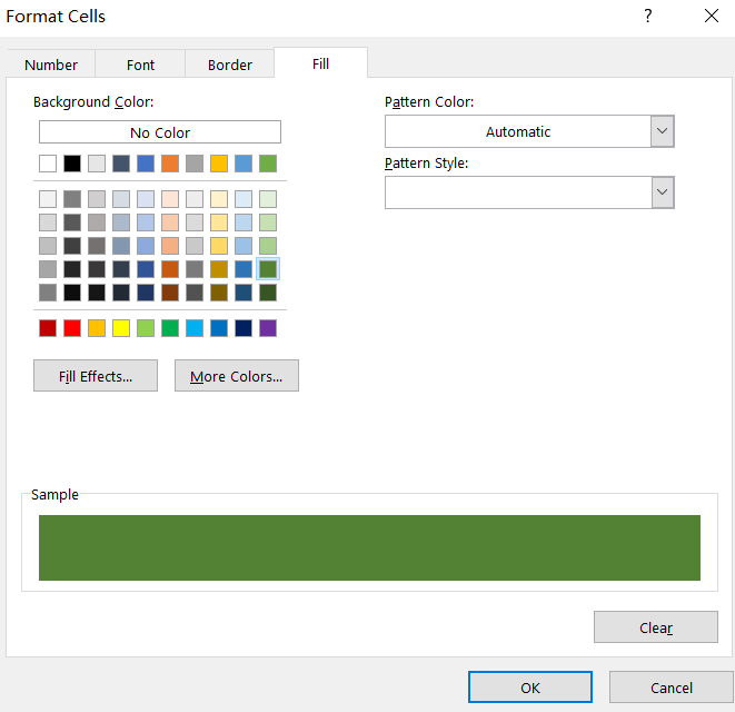
Step6: click Format button, and the Format Cells dialog will open. Click Fill tab, select on color that you want to use. Click Ok button.

Step7:  click Ok button.

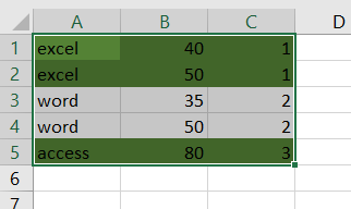
If you want to alter row color for Even rows, you just need to add another New Rule with a formula based on the ISEVEN($C1). so you just need to repeat the above steps.

=ISEVEN($C1)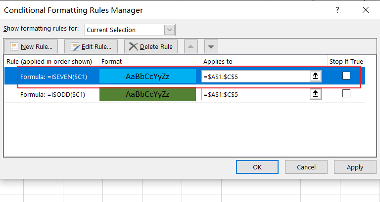

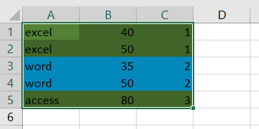
2. Video: Alternating Rows Color by Groups

This tutorial video, where we’ll delve into the world of conditional formatting and explore how to apply alternate row colors based on specific groups in your data in Excel.