If you are a frequent user of Google Spreadsheets, you may have come across situations where you needed to add or count the cells that were case-sensitive. If you have done this task manually, I would like to point out that it is the most inefficient way to do it, particularly when Google Spreadsheets has the versatility to do it in a matter of seconds. As a result of attentively reading this article, you will learn about the many adding or counting case-sensitive cells.

Simple generic formula:

=SUMPRODUCT(--ISNUMBER(FIND(value, range)))

Summary

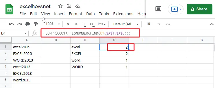
You may use a formula depending on the ISNUMBER and FIND functions and the SUMPRODUCT function to calculate the number of cells that contain specified text (i.e., hold a substring), taking into consideration upper and lower case. D1 in the example displayed has the following formula, which has been written down:

=SUMPRODUCT(--ISNUMBER(FIND(C1,$A$1:$A$6)))

Let’s See How This Formula Works

In this example, the purpose is to count the number of times each code appears as a substring in a case-sensitive manner, as shown below. When calculating text values, the functions COUNTIF and COUNTIFS are excellent choices. However, since these functions are not case-sensitive, they cannot be utilized to address this issue. To check for substrings, the FIND function should be used in conjunction with the ISNUMBER function, and the SUMPRODUCT function should be used to sum up, the results.

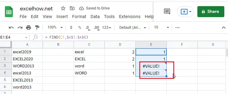
= FIND(C1,$A$1:$A$6)

The FIND function is case-sensitive and accepts three parameters: find text, within the text, and start num. It is also case-sensitive and takes three arguments. Here is the text we are searching for, and this is the text that we are searching inside. Start num is the number of characters to begin searching in find text. Because start num defaults to 1, we are not supplying a number in this instance. This is necessary since we always want FIND to begin with the first character. When finding the text is discovered inside within text, FIND returns the position of the found text as a number: When finding the text is located within text, FIND returns the position of the found text as a number:

Note: When the find text function fails to yield a result, FIND returns the #VALUE! Error.

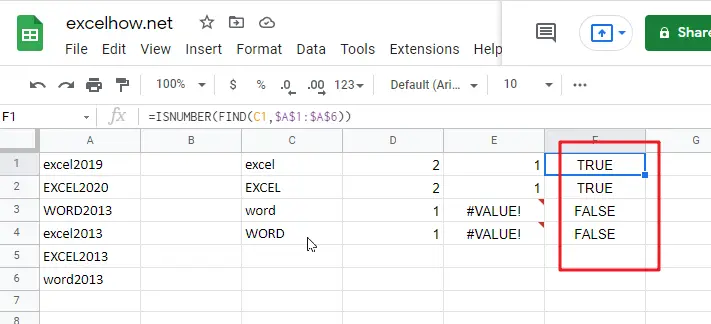
=ISNUMBER(FIND(C1,$A$1:$A$6))

This implies that we may be using the ISNUMBER function to transform the output of the FIND function into a TRUE or FALSE value using the ISNUMBER function. A TRUE value will arise from any number, while a FALSE value will result from any error:

As demonstrated in the example, we have four substrings in column C and a variety of codes in columns A1:A6, representing the data for the designated range. Specifically, we want to know how many times each substring in C1:C4 occurs in A1:A6, and we want to know how many times each substring is case-sensitive.

Related Functions

• Excel ISNUMBER function
  The Excel ISNUMBER function returns TRUE if the value in a cell is a numeric value, otherwise it will return FALSE.The syntax of the ISNUMBER function is as below:= ISNUMBER (value)…
• Google Sheets FIND function
  The Google Sheets FIND function returns the position of the first text string (sub string) within another text string.The syntax of the FIND function is as below:= FIND(find_text, within_text,[start_num])…
• Google Sheets SUMPRODUCT function
  The Google Sheets SUMPRODUCT function multiplies corresponding components in the given one or more arrays or ranges, and returns the sum of those products.The syntax of the SUMPRODUCT function is as below:= SUMPRODUCT (array1,[array2],…)…
• Google Sheets COUNTIF function
  The Google Sheets CHOOSE function returns a value from a list of values based on index. The syntax of the CHOOSE function is as below:=CHOOSE (index_num, value1,[value2],…) …
• Google Sheets COUNTIFS function
  The Google SheetsCOUNTIFS function returns the count of cells in a range that meet one or more criteria. The syntax of the COUNTIFS function is as below:= COUNTIFS(criteria_range1, criteria1, [criteria_range2, criteria2]…)…