This post will guide you how to count unique items in Excel Pivot Table. How do I use Pivot Table to count unique distinct values in Excel. How to get a distinct count in a pivot table in Excel.

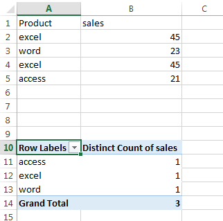
Assuming that you have a list of 5 cells with 3 unique values, and you want to create an excel pivot table to count unique values, how to achieve it. You can insert a 3rd or helper column to check if the value is unique in the selected range of cells, and the create pivot table based on the 1st and 3rd column to count unique values. Or you can use the Distinct Count feature in pivot table to achieve the result, but this feature is only available in Excel 2013 and Excel 2016 version.

1. Count Distinct Values Using Pivot Table with help column

#1 Insert 3rd column named as helper column (Column C), then type this formula into the Cell C2.

=IF(SUMPRODUCT(($A$2:$A2=A2)*($B$2:$B2=B2))>1,0,1)

#2 press Enter key in your keyboard, and drag the AutoFill Handler over other cells in helper column to apply this formula. If the returned value is 1, then it indicated that the value is the first value, if it returns 0, it indicated that the value is a duplicated value.

#3 select the data to be included in a pivot table, the helper column should be also included.

#4 go to INSERT tab, click the PivotTable command under Tables group. The create PivotTable dialog will appear.

#5 select Existing Worksheet radio button, and then select one cell or range to place the PivotTable report. Click OK button.

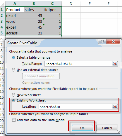
#6 choose fields to add to report in PivotTable fields pane. Choose Product and Helper fields checkbox.

#7 let’ see the result.

2. Count Distinct Values Using Pivot Table with distinct Count Feature

If you are using the latest version of Excel 2013 or Excel 2016, there is a new feature to allow you to count distinct values automatically in the pivot table. Let’s see the below detailed steps:

#1 select the range of cells that you want to be added into pivot table.

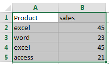
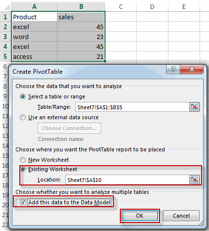
#2 Click “INSERT” in the Ribbon tab, then clicking “Pivot Table” button in the “Tables” group. The Create PivotTable dialog will appear.

#3 select Existing Worksheet radio button, and then select one cell or range to place the pivottable report. and select the Add this data to the Data Model checkbox. Click OK button.

#4 arrange the Rows, Columns and Values areas by dragging fields in PivotTable Fields pane.

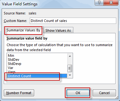
#5 click on Values area, and select Value Field Settings from the drop down list. The Value Field Settings dialog will open.

#6 click Summarize Values By tab, and scroll down to Distinct Count, then click OK button.

#7 Let’s see the result.

3. Video: Count Distinct Values Using Pivot Table

This Excel video tutorial, we’ll explore two methods to count unique values using a Pivot Table. We’ll start by utilizing a help column combined with a formula approach, followed by leveraging the distinct count feature.

4. Related Functions

• Excel SUMPRODUCT function
  The Excel SUMPRODUCT function multiplies corresponding components in the given one or more arrays or ranges, and returns the sum of those products.The syntax of the SUMPRODUCT function is as below:= SUMPRODUCT (array1,[array2],…)…
• Excel IF function
  The Excel IF function perform a logical test to return one value if the condition is TRUE and return another value if the condition is FALSE. The IF function is a build-in function in Microsoft Excel and it is categorized as a Logical Function.The syntax of the IF function is as below:= IF (condition, [true_value], [false_value])….