This post will guide you how to create a chart that updates with new data automatically in Excel. How do I create self-updating chart in Excel. How to get charts to automatically update with new data point in your current worksheet. Or how to use defined names to update a chart with new data point automatically in Excel.

Assuming that you have a list of data and you have created a column chart based on these data. And you want to add one row or data point in the original data source, and you also want the existing column chart can be updated automatically. How to achieve it. This post will introduce two methods to update chart automatically.

1. create a table based on the original source data

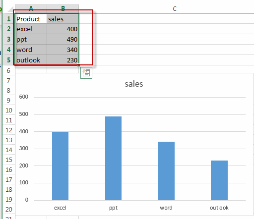
You can create a new table based on the source data of the chart, then you can add one row data point under the created table. And you will find that the newly added data point will be updated to the current column chart. Just do the following steps:

#1 select the source data in your worksheet.

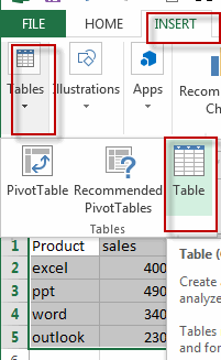
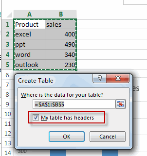
#2 go to INSERT tab, click Table command under Tables group. The Create Table dialog will open. If you data has headers and you need to select My table has headers checkbox.  Click OK button.

#3 the table has been created based on the selected range of cells.

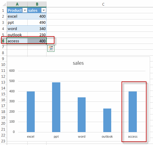
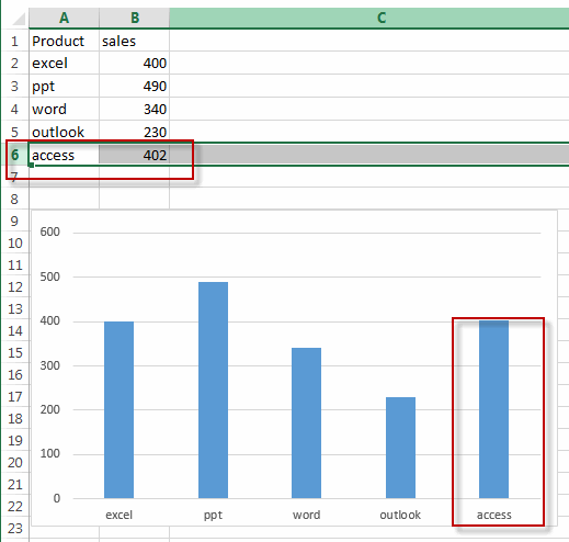
#4 add one data point under the table. And the newly added data is added into the current column chart automatically.

2. Use Defined Name to Update the Chart Automatically

You can also use the defined name for each column to update the chart with new data point automatically. Just do the following steps:

#1 Go to FORMULAS tab, click Define Name command under Defined Names group to create one defined name for each column.

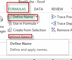
#2 Enter Product in the Name text box, and type the following formula into the Refers to text box.

=OFFSET($A$2,0,0,COUNTA(Sheet1!$A:$A)-1)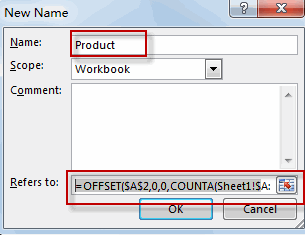

#3 repeat the step 2 to create defined name for Sales column. Type the following formula into the Refers to text box.

=OFFSET($B$2,0,0,COUNTA(Sheet1!$B:$B)-1)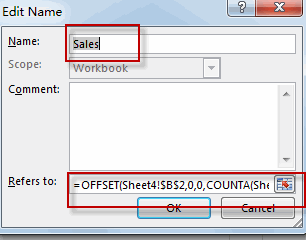

#4 click on the chart ,and the click any data series in your chart. Changing the current formula in the formula bar to the following formula. Then press Enter key.

=SERIES(,Sheet1!Product,Sheet1!Sales,1)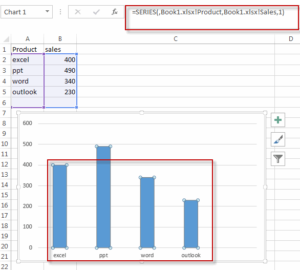

#5 add one new data under the source data. The chart will update automatically for the newly added data point。

3. Video: Create a Chart That Updates with New Data Automatically

This Excel video tutorial where we’ll unravel the methods of creating dynamic charts that effortlessly adapt to new data. In this session, we’ll explore two powerful techniques – creating tables and utilizing the defined name feature.

4. Related Functions

• Excel COUNTA function
  The Excel COUNTA function counts the number of cells that are not empty in a range. The syntax of the COUNTA function is as below:= COUNTA(value1, [value2],…)…