This post will guide you how to create a dynamic drop down list in Excel. How do I quickly create a dynamic drop down list in Excel.

Create Dynamic Drop Down List

---

Assuming that you want to create two drop down list in your current worksheet, and when choose a value in one drop down list, and the values in another drop down list will be updated automatically. How to achieve it. Let’s see the below detailed steps.

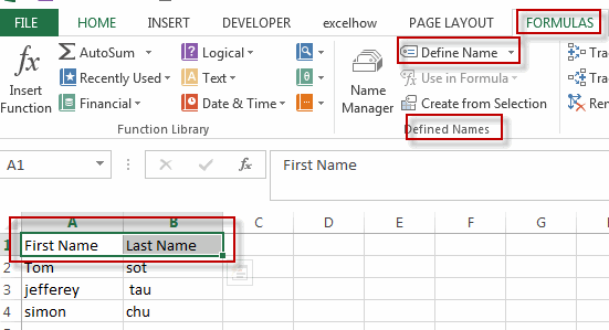
#1 select the range of cells A1:B1, go to FORMULAS tab, click Define Name command under Defined Names group. The New Name dialog will open.

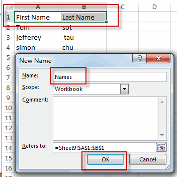
#2 type one Name in the Name text box. Then click OK button.

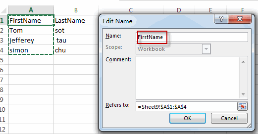
#3 select the range of cells A1:A4 to create another defined name.

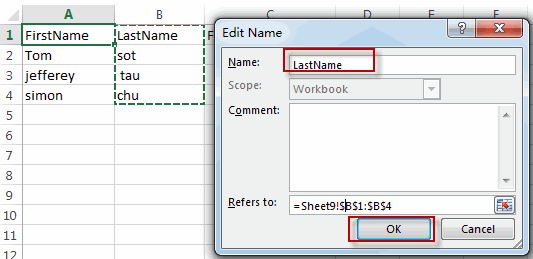
#4 select the range of cells B1:B4 to create one more defined name.

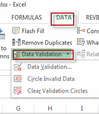
#5 create the first drop down list, go to DATA tab, Click Data Validation command under Data Tools group. And select Data Validation item from the pop up menu list. The Data Validation dialog will open.

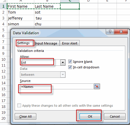
#6 click Settings tab, select List from the Allow drop down list box. And type the formula =Names in the source text box. Click Ok button.

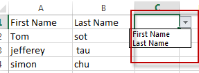
#7 the first drop-down list has been created in Cell C1.

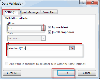
#8 click Cell D1 to select this cell, go to DATA tab, Click Data Validation command under Data Tools group to create the second drop down list. Click Settings tab, select List from the Allow drop down list box. And type the formula =indirect(C1) in the source text box. Click Ok button.

#9 choose one value from the first drop down list, and you will see that the values in the second drop down list will be updated.