This post will guide you how to use Excel HYPERLINK function with syntax and examples in Microsoft excel.
Table of Contents
Description
The Excel HYPERLINK function creates a shortcut/hyperlink to a document, when you click this hyperlink, the excel will open the file that is stored on a network server or local location.
The HYPERLINK function is a build-in function in Microsoft Excel and it is categorized as a Lookup and reference Function.
The HYPERLINK function is available in Excel 2016, Excel 2013, Excel 2010, Excel 2007, Excel 2003, Excel XP, Excel 2000, Excel 2011 for Mac.
Syntax
The syntax of the HYPERLINK function is as below:
= HYPERLINK(link_location,[friendly_name])
Where the HYPERLINK function arguments are:
Link_location -This is a required argument. A link path to a file that you want to hyperlink.
Friendly_name-This is an optional argument. The text string to display in the excel cell.
Note: If the link_location does not exist or cannot be navigated, error will appear when you click the hyperlink text.
Example
The below examples will show you how to use Excel HYPERLINK Lookup function to create a hyperlink text to a file.
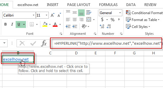
#1 To create a hyperlink text with “excelhow.net” friendly name, with “http://www.excelhow.net” link as link_Location in B1 cell , just using the following formula:=HYPERLINK(“https://www.excelhow.net”,”excelhow.net”).

Leave a Reply
You must be logged in to post a comment.