This post will guide you how to use Excel IFERROR function with syntax and examples in Microsoft excel.

Description

The Excel IFERROR function returns an alternate value you specify if a formula results in an error, or returns the result of the formula.

The IFERROR function is a build-in function in Microsoft Excel and it is categorized as a Logical Function.

The IFERROR function is available in Excel 2016, Excel 2013, Excel 2010, Excel 2007, Excel 2003, Excel XP, Excel 2000, Excel 2011 for Mac.

Syntax

The syntax of the IFERROR function is as below:

= IFERROR (value, value_if_error)

Where the IFERROR function arguments are:

• Value -This is a required argument. The value or formula that you want to test
• Value_if_error – This is a required argument.  The value that is returned if the formula evaluates to an error.  The below errors will check: #VALUE!, #N/A, #REF!, #DIV/0!, #NUM!, #NAME?, or #NULL!.

Example

The below examples will show you how to use Excel IFERROR Function to return an alternate value if a formula evaluates to an error.

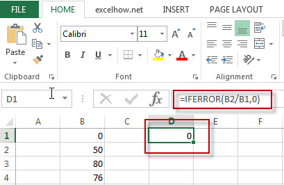
#1 =IFERROR(B2/B1,0)

Note: the formula “B2/B1” will return an #DIV/0! Error,  if you use “IFERROR” function, the above excel formula will return an alternate value 0.

More IFERROR Function Examples

• remove non numeric characters from a cell
  If you want to remove non numeric characters from a text cell in excel, you can use the array formula:{=TEXTJOIN(“”,TRUE,IFERROR(MID(B1,ROW(INDIRECT(“1:”&LEN(B1))),1)+0,””))}…
• Get the List of File Names From a Folder
  You will learn that how to use Excel to view Files and Folders in your worksheet by get the list of file names with different ways, such as: Excel VBA Macro, or FILES function.…
• Extract a List of Unique Values from a Column Range
  If you want to extract a list of unique items from a column or range, you can use a combination of the IFERROR function, the INDEX function, the MATCH function and the COUNTIF function to create an array formula.…
• Extract multiple match Values into different Columns or Rows
  If you want to fetch all matches from a range then put it into cells in different columns, you can use a combination with the INDEX function, the SMALL function, the IF function,  the ROW function and the COLUMNS function to create a new excel formula..…
• VLOOKUP Values from Multiple Worksheets
  you can use the VLOOKUP function to find the values from multiple worksheets in Excel. For example, assuming that you have two worksheets, and you want to search the data across those two worksheet in your current worksheet (sheet3)……