This post will guide you how to use Excel MATCH function with syntax and examples in Microsoft excel.

Description

The Excel MATCH function search a value in an array and returns the position of that item.

The MATCH function is a build-in function in Microsoft Excel and it is categorized as a Lookup and Reference Function.

The MATCH function is available in Excel 2016, Excel 2013, Excel 2010, Excel 2007, Excel 2003, Excel XP, Excel 2000, Excel 2011 for Mac.

Syntax

The syntax of the MATCH function is as below:

= MATCH  (lookup_value, lookup_array, [match_type])

Where the MATCH  function arguments are:
Lookup_value -This is a required argument.  The value that you want to search.
Lookup_array – This is a required argument.  The data array that is to be searched.
Match_type – This is an optional argument.  This value can be set as: 1, 0, -1. The default value is 1.

Note:  
1 – the MATCH function will search the largest value that is less than or equal to Lookup_value
0 – The MATCH function will search the first value that is exactly equal to Lookup_value
-1 – The Match function will search the smallest value that is greater than or equal to Lookup_value.

Example

The below examples will show you how to use Excel MATCH  Lookup and Reference Function .

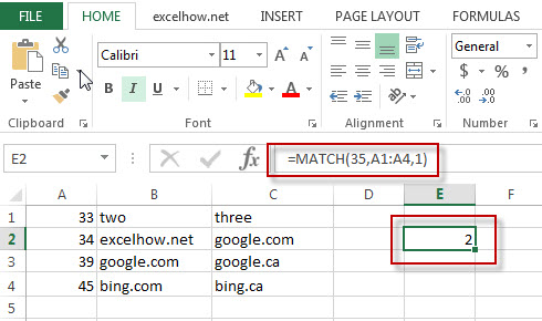
#1 =MATCH(35,A1:A4,1)

This Excel Formula will lookup the value “35” and find the largest value that is less than or equal to “35”, it will return “2”, As the value “34” is the only  largest value that is less than to “35”. So it will return the position of value “34” in range “A1:A4”.

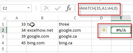
#2 =MATCH(35,A1:A4,0)

This Formula will return the “#N/A” value, As the Match type is set to “0”, it means that the function will find the first value that is exactly equal to “35”, but it is not able to find the value “35” in “A1:A4” range.

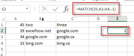
#3 =MATCH(35,A1:A4,-1)

This Formula will return “2”, if the Match type is set to “-1”, the Match function will find the smallest value that is greater than or equal to “35”in range “A1:A4”, then return its position.

More Excel MATCH Formula Examples

---

• Finding the Max and Min value in an Alphanumeric Data
  if you want to find the Maximal or minimal string value from an alphanumeric data list in the range B1:B5, you can create a formula based on the LOOKUP function and the COUNTIF function.….
• Convert Weekday Name to Number
  Assuming that you have list of data B1:B7 that contain weekday names, you want to convert all weekday names to numbers.You can use a formula based on the MATCH function to achieve the result
• Find Missing Numbers in a Sequence in Excel
  You can use an excel array formula based on the SMALL function, the IF function, the ISNA function, the MATCH function, and the ROW function to find missing numbers in a sequence…
• Find Closest Value or Nearest Value in a Range
  You need to use an excel array formula based on the INDEX function, the MATCH function, the MIN function and the ABS function to find Closest Value or Nearest Value in a Range in Excel…