This post will guide you how to use the RANK function with syntax and examples in Microsoft excel.

Description

The Excel RANK function returns the rank of a given number in a supplied range of cells.  If there are duplicated values in a list of values, it will be set the same rank. This function has been replaced by the RANK.EQ function in Excel 2010.

The RANK function is a build-in function in Microsoft Excel and it is categorized as a Statistical Function.

The RANK function is available in Excel 2016, Excel 2013, Excel 2010, Excel 2007, Excel 2003, Excel XP, Excel 2000, Excel 2011 for Mac.

Syntax

The syntax of the RANK function is as below:

= RANK (number,ref,[order])

Where the RANK function arguments are:

• Number – This is a required argument.  The number for which you want to get the rank.
• ref – This is a required argument. An array or range of cells, or cell reference that contain the supplied number.
• Order – This is an optional argument. . A number specifying how to rank number. If order is 0 or omitted, the RANK function will rank the numbers in descending order. If the order is not equal to 0, the RANK function will rank numbers in ascending order.

Excel RANK Function Examples

The below examples will show you how to use Excel RANK Function to get the rank of a given value within a supplied range of cells.

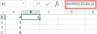
Example 1:  to get the rank of 4 in a given range of cells (A1:A4), using the following formula:

=RANK(5,A1:A4,1)

More Excel Rank Function Examples

---

• Rank Data with Multiple Criteria
  Assuming that you want to rank data against multiple criteria for a range of cells in your worksheet. How to achieve it. You need to create a new complex formula based on the SUMPRODUCT function. .…
•  Rank values in a column based a specific value in another column
  Assuming that you have a list of data contains two columns and the first column is product list and another is Sales number. You want to rank the sales number of a specified product name. You can try to write a complex formula based on the IF function and the COUNTIFS function to achieve the result..…
• Reverse Rank Order
  Assuming that you have a formula based on RANK function that ranks numbers by biggest to smallest by default. But you want to go the opposite from the smallest to biggest.…
• Rank data Based on the Number of Occurrences
  You need to get the number of occurrences for the selected range of cells, then rank those number using the RANK function…