The use of Microsoft Excel’s Format Cells and Auto Filter option is a great way to filter data by year or Month. This article will discuss how to filter by date field using Filter function and Format cells in Microsoft excel.

Filter Data by Date Field using FILTER Function

The General Formula is as below:

=FILTER(Total_data,MONTH(range2)=5,"Not Found")

Summary

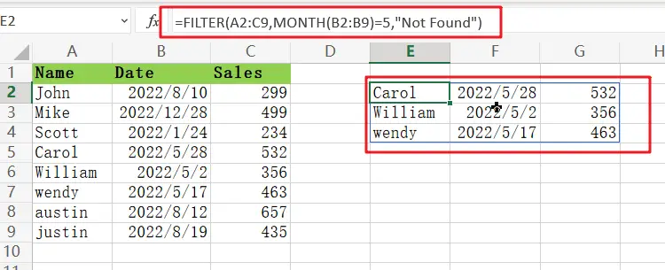
FILTER function can be used with one of Excel’s date functions to make your data more relevant. In this example shown below, E2 is used:

=FILTER(A2:C9,MONTH(B2:B9)=5,"Not Found")

This is a great way to only show data from one specific Month. For example, it would be easy to want our report for May only! We need to get this effect out of the filter engine. (A2:C9) and then add “date” after that with B2:B9 named ranges, so no other periods show up when looking through your findings.

Clarification:

The MONTH function is used to create an argument for the FILTER function that filters based on a logical test created with ONE of many other functions available in Excel. The array data contains all information, without any headers or spaces between values, perfect if you want every record exactly how it’s shown!

=MONTH(B2:B9)

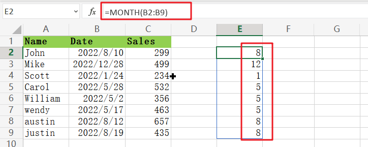
Month contains a range from B2:B9. Since this is an array with 8 cells, MONTH returns 8 results!

=MONTH(B2:B9)=5

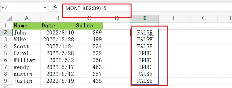
The “include” argument is a set of values determining which results will be included in the array. These are compared to 5, and this operation creates an ordered list with TRUE or FALSE as its elements before delivering it on through filter function call.

Only when the result is TRUE will it appear in this final output. The “if_empty” argument has been set to ‘ Not Found ‘ so as not to show any unmatched records or values.”

Filter By Month And Year

To filter by Month and year, use the following formula:

=FILTER(A2:C9,(MONTH(B2:B9)=5)*(YEAR(B2:B9)=2022),"Not Found")

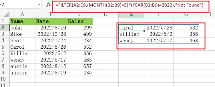
The values for Month and year can easily be replaced with cell references.

Filter the Data by Date using Format Cell

Now we’ll look at how to filter the data by date. We have information in range A1: C9, with dates represented as columns on each line representing who purchased what from us over time.

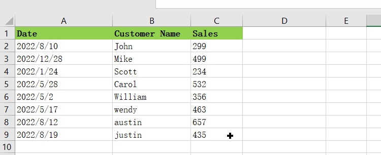
To change the filter for a specific month or year, follow these steps:

Step1: Copy A1:A9 and paste it right next to column A

Step2: Click on the range A1:A9 and select

Step3: To copy the date, press Control+C on your keyboard.

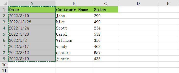
Step4: Select cell A1 and press Ctrl+Shift+”+”

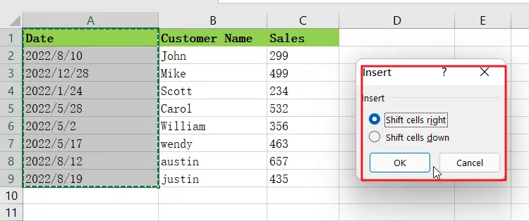
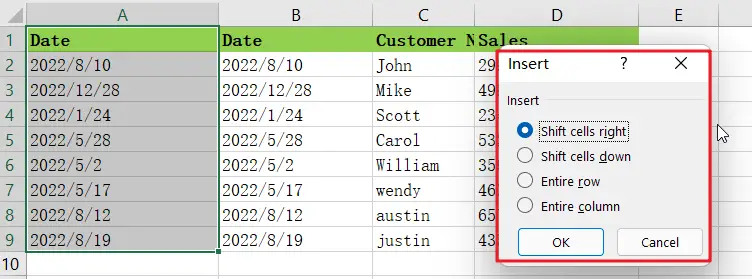
Step5: The Insert Dialog Box will appear.

Step6: To continue editing the data, choose Shift Cells right and click the Ok button.

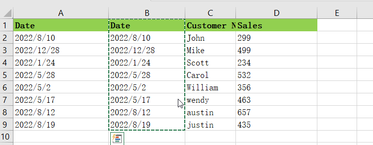
Step7: To increase the range of cells that you can paste into, copy and then press Ctrl+ shift +. Then select shift cells right in the insert dialog box by clicking OK.

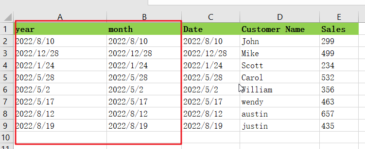
Step8: A new month and year are just around the corner, so it’s time to update your headlines!

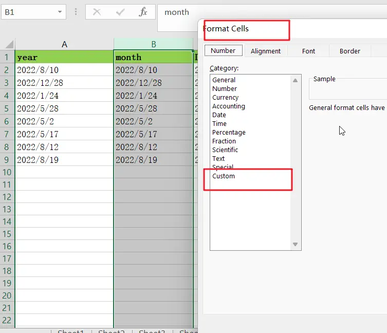
Step9: Select the column of Month and then press ctrl+1 keys to open the format cells dialog box

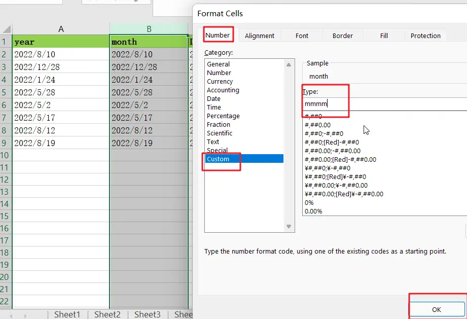
Step10: Once the dialog box appears, then select custom in the number tab.

Step11: Enter mm (to show Month’s full name) in the type box and click on OK.

Step12: Now select the Column of Year and press the Ctrl+1 to open the format cells dialog box.

Step13: Once the dialog box appears, select custom in the number tab.

Step14: In order to show the full year, just enter YYYY in this box and click on.

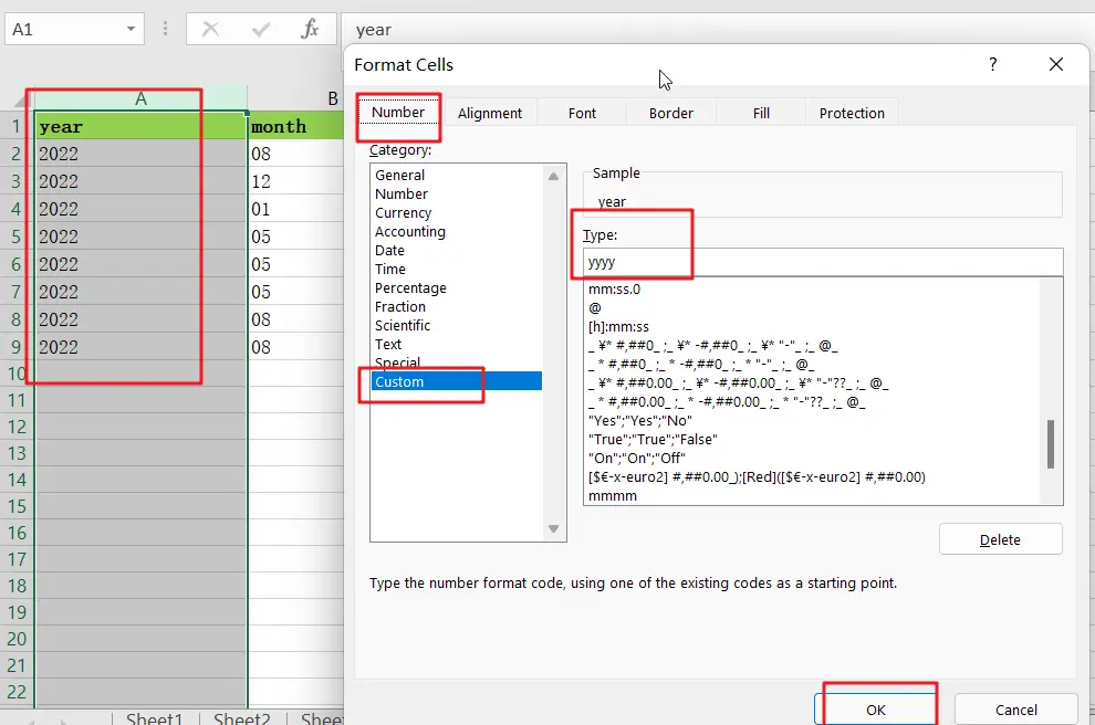
Step15: The output is a simple list that can be sorted by either Month or year.

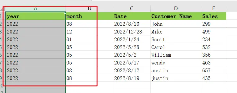
Step16: You can also use this trick to filter any cell quickly. Select the desired range and press Ctrl+Shift+L.

If you want to filter the data according to a specific month or year, select cell A1 and press Ctrl+Shift+L.

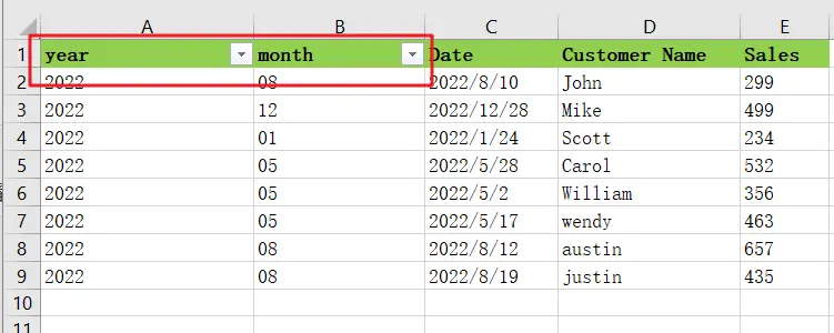
Conclusion:

We’ve given you the tools to filter your data in Microsoft Excel by date fields in this blog post. Now that you know how easy it is to do, why not try adding a few more filters to your workbook? You may be surprised what insights can come from applying multiple filters at once!

Related Functions

• Excel Filter function
  The Excel  FILTER function extracts matched records from a collection of data using one or more logical checks. The include argument specifies logical tests, which might encompass a wide variety of formula conditions.==FILTER(array,include,[if empty])…
• Excel MONTH Function
  The Excel MONTH function returns the month of a date represented by a serial number. And the month is an integer number from 1 to 12.The syntax of the MONTH function is as below:=MONTH (serial_number)…
• Excel YEAR function
  The Excel YEAR function returns a four-digit year from a given date value, the year is returned as an integer ranging from 1900 to 9999. The syntax of the YEAR function is as below:=YEAR (serial_number)…