This tutorial will show you how to find duplicate values in two given columns in Excel. Or How to compare two columns and find duplicate entries in Microsoft Excel worksheet. And you will learn two methods to compare columns so that the duplicate values can be highlighted or listed in a range of Cells.

Assuming that you need to compare two columns (Column A and Column B) to get the duplicate values in your worksheet, you can find duplicate values in two columns with Excel Formula, or Excel VBA Macro code.

1. Find duplicate values in two columns with Excel Formula

To compare two given columns and find duplicate values in Excel, you can use a combination of the IF function, the ISERROR function, and the MATCH function to create an Excel formula. So you can use the following formula:

=IF(ISERROR(MATCH(A1,$B$1:$B$4,0))," ",A1)

Now you need to type this formula in Cell C1, press Enter key, drag AutoFill Handle down to Cell C2:C4, you will see all of the duplicated values are displayed in Column C.

2. Find duplicate values in two columns with VBA Macro code

If you are familiar with the programming language and you can use a Visual Basic Macro to compare the value in two columns and then find duplicate values, just refer to the following steps:

1# click on “Visual Basic” command under DEVELOPER Tab.

2# then the “Visual Basic Editor” window will appear.

3# click “Insert” ->”Module” to create a new module

4# paste the below VBA code into the code window. Then clicking “Save” button.

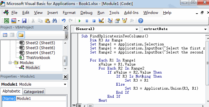
Sub FindDuplicatesInTwoColumns()
    ' Define the range for the first column
    Set Range1 = Application.Selection
    ' Prompt user to select the first range in one column
    Set Range1 = Application.InputBox("Select the first range in one column:", "FindDuplicatesInTwoColumns", Range1.Address, Type:=8)
    
    ' Prompt user to select the second range in another column
    ' Note: The second input box does not have a default address, so we can remove the third parameter
    Set Range2 = Application.InputBox("Select the second range in another column:", "FindDuplicatesInTwoColumns", Type:=8)
    
    Dim R3 As Range
    ' Initialize R3 to Nothing
    Set R3 = Nothing
    
    ' Loop through each cell in the first range
    For Each R1 In Range1
        Dim xValue As Variant
        xValue = R1.Value
        ' Loop through each cell in the second range
        For Each R2 In Range2
            If xValue = R2.Value Then
                If R3 Is Nothing Then
                    ' Set R3 to the first duplicate cell found
                    Set R3 = R1
                Else
                    ' Union R3 with the current cell if it's not the first duplicate
                    Set R3 = Application.Union(R3, R1)
                End If
            End If
        Next R2
    Next R1
    
    ' If duplicates were found, color the cells
    If Not R3 Is Nothing Then
        R3.Interior.ColorIndex = 3
    End If
End Sub

5# back to the current worksheet, then run the above excel macro.

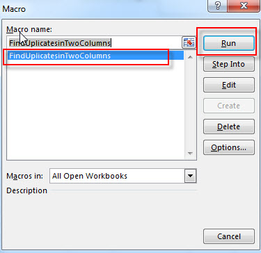
6# Select the first range A1:A4 in Column A, click OK button, then select the second range B1:B4 in Column B, click OK button.

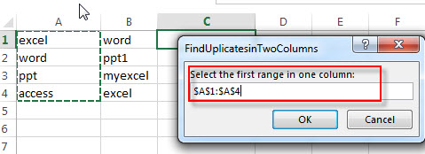
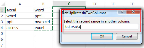
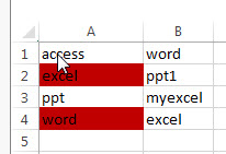
7# let’s see the result:

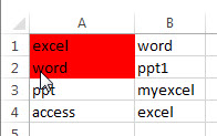
3. Find duplicate values in two columns with Conditional Formatting feature

You can use conditional formatting with on a formula based on the COUNTIF function and the AND function to find the duplicate values in two specified columns and then highlighted them. Just do it following:

1# Select the entire Column A via click on the Column Header and then the column A will be highlighted

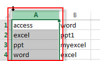
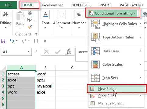
2# on the HOME tab, click the Conditional Formatting command under Styles group. Then select New Rules… from the drop-down menu list.

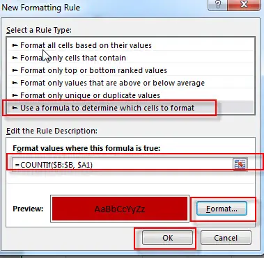
3# select Use a formula to determine which cells to format as Rule Type in the New Formatting Rule window

4# Type the following formula in the Format values where this formula is true: box

=COUNTIf($B:$B, $A1)

5# click the Format… button, then the Format Cells window will appear.

6# in the “Format Cells” window, switch to the Fill tab, choose the background color, and then click OK button.

7#you will be back to the New Formatting Rule windows and you can check a preview of the formatting you have selected. Then click OK button.

Then the conditional formatting rule will be applied to all values in two columns and highlighted the duplicate values.

4. Video: Find duplicate values

This Excel video tutorial, we’re going to explore how to find duplicate values in two given columns using various methods. Whether you’re using Excel formulas, VBA macros, or conditional formatting, these techniques will help you quickly identify and manage duplicate data in your spreadsheets.

5. Related Functions

• Excel IF function
  The Excel IF function perform a logical test to return one value if the condition is TRUE and return another value if the condition is FALSE. The IF function is a build-in function in Microsoft Excel and it is categorized as a Logical Function.The syntax of the IF function is as below:= IF (condition, [true_value], [false_value])….
• Excel ISERROR function
  The Excel ISERROR function used to check for any error type that excel generates and it returns TRUE for any error type, and the ISERR function also can be checked for error values except #N/A error, it returns TRUE while the error is #N/A. The syntax of the ISERROR function is as below:= ISERROR (value)….
• Excel MATCH function
  The Excel MATCH function search a value in an array and returns the position of that item.The syntax of the MATCH function is as below:= MATCH  (lookup_value, lookup_array, [match_type])….
• Excel COUNTIF function
  The Excel COUNTIF function will count the number of cells in a range that meet a given criteria. This function can be used to count the different kinds of cells with number, date, text values, blank, non-blanks, or containing specific characters.etc.= COUNTIF (range, criteria)…
• Excel AND function
  The Excel AND function returns TRUE if all of arguments are TRUE, and it returns FALSE if any of arguments are FALSE.The syntax of the AND function is as below:= AND (condition1,[condition2],…)…

6. Related Posts

• Highlight Rows
  You will learn that how to change the color of the entire rows if the value of cells in a specified column meets your conditions, such as, if the value of cells is equal to or greater than a certain number or text values, then excel should be highlight entire rows or change a row color as you need.…
• Find Duplicate Rows
  If you want to check the entire row that duplicated or not, if True, then returns “duplicates” value, otherwise, returns “no duplicates”. You can create a formula based on the IF function and the SUMPRODUCT function..…
• Highlight Duplicate Rows
  this post will talk that how to highlight entire rows that are duplicates in excel 2016, 2013 or lower version. Or how to change the background color of duplicate rows..…
• Highlight duplicate values
  this post will teach you how to highlight duplicate values in the range of cells in excel. Normally, you may be need to identify duplicate values with a range of cells in Excel. And there is one of the fasted way that is using conditional formatting feature in Microsoft Excel……