This post will guide you how to flip a column of data vertically preserving the original formatting and formulas in Excel. How do I reverse a column of data order in a column arranged alphabetically or from largest to smallest. How to use the Excel Sort feature to reverse the data order? Or how to use a VBA macro code to flip a column of data vertically in Excel.

If you want to flip or reverse a column of data that is already in numeric or alphabetical order, and you can easily to flip it with Sort feature. And if the column data is not sorted and you can try to create a helper column to achieve the result.

1. Flip a Column of Data with Sort Feature

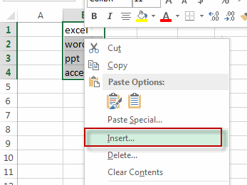
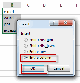
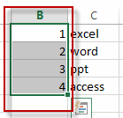
#1 select the column that you want to flip, right click on it, and select Insert to add helper column. Choose Entire column radio button. Then insert 1,2,3,4,…in helper column.

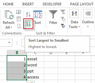
#2 select your helper column, then go to the Data tab, click the Sort Largest to Smallest command under Sort&Filter group.

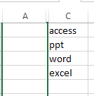
#3 you will see that the numbers in help column will be sorted and the data of column also be reversed. Now you can delete the help column. Or you can also hide the help column in case you want to restore the data of column.

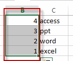
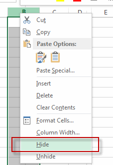
#4 let’s see the result

2. Flip a Column of Data Vertically with Function

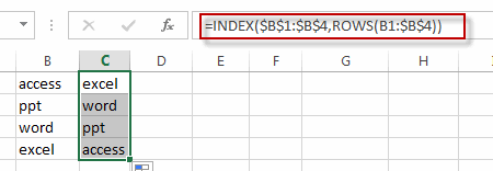
You can also create an excel formula based on the INDEX function and the ROWS function to flip a column of data vertically. Type the following formula in the formula box of cell C1, then press enter key.

=INDEX($B$1:$B$4,ROWS(B1:$B$4))

Let’s see the result as below:

3. Flip a Column of Data Vertically with VBA Macro

You can also write an Excel VBA Macro to flip a column of data vertically quickly. Just do the following steps:

#1 click on “Visual Basic” command under DEVELOPER Tab.

#2 then the “Visual Basic Editor” window will appear.

#3 click “Insert” ->”Module” to create a new module.

#4 paste the below VBA code into the code window. Then clicking “Save” button.

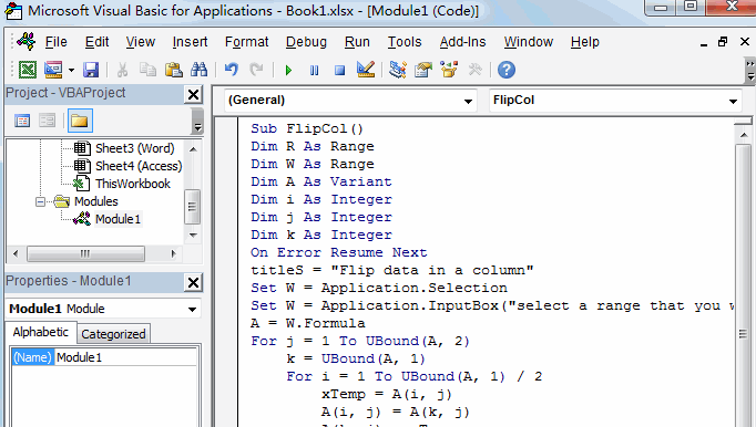
Sub FlipCol()
    Dim R As Range
    Dim W As Range
    Dim A As Variant
    Dim i As Integer
    Dim j As Integer
    Dim k As Integer
    On Error Resume Next
    titleS = "Flip data in a column"
    Set W = Application.Selection
    Set W = Application.InputBox("select a range that you want to reverse", titleS, W.Address, Type:=8)
    A = W.Formula
    For j = 1 To UBound(A, 2)
        k = UBound(A, 1)
        For i = 1 To UBound(A, 1) / 2
            xTemp = A(i, j)
            A(i, j) = A(k, j)
            A(k, j) = xTemp
            k = k - 1
        Next
    Next
    W.Formula = A
End Sub

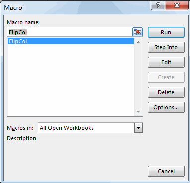
#5 back to the current worksheet, then run the above excel macro. Click Run button.

#6 select a range that you want to flip.

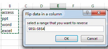
#7 click OK button, then check the result.

4. Video: Flip a Column of Data Vertically

This Excel video tutorial, we’ll explore three methods to flip a column of data vertically. We’ll start by using a formula with the INDEX and ROWS functions, followed by leveraging the Sort feature, and finally, we’ll delve into a VBA Macro.

https://youtu.be/1XOaM2tIp_4

5. Related Functions

• Excel INDEX function
  The Excel INDEX function returns a value from a table based on the index (row number and column number)The INDEX function is a build-in function in Microsoft Excel and it is categorized as a Lookup and Reference Function.The syntax of the INDEX function is as below:= INDEX (array, row_num,[column_num])…
• Excel ROWS function
  The Excel ROWS function returns the number of rows in a cell reference.The syntax of the ROWS function is as below:= ROWS(array)…