This post will guide you how to generate all possible combinations with a formula in excel. How do I create list with all possible combinations of two lists in Excel. How to list all combinations from two separate list or range in Excel.
Table of Contents
1. Generate All Possible Combinations of Two Lists using Formula
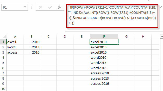
Assuming that you have two list of data in different column, A and B, and you want to get a list of all possible combinations from those two list in Column A and B. How to achieve it.
You can use a formula based on the IF function, the ROW function, the COUNTA function, The INDEX function and the MOD function. Like this:
=IF(ROW()-ROW($F$1)+1>COUNTA(A:A)*COUNTA(B:B),"",INDEX(A:A,INT((ROW()-ROW($F$1))/COUNTA(B:B)+1))&INDEX(B:B,MOD(ROW()-ROW($F$1),COUNTA(B:B))+1))Type this formula into Cell F1, and then drag the AutoFill Handle down column F until you get cells that look empty.

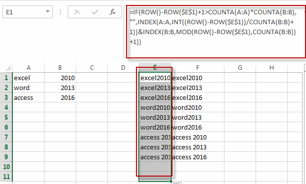
Note: if you want to use this formula into other cell, you need to change the absolute cell reference to that cell. Such as: form F1 to E1.
=IF(ROW()-ROW($E$1)+1>COUNTA(A:A)*COUNTA(B:B),"",INDEX(A:A,INT((ROW()-ROW($E$1))/COUNTA(B:B)+1))&INDEX(B:B,MOD(ROW()-ROW($E$1),COUNTA(B:B))+1))
2. Creating All Possible Combinations Using VBA Code
You can also create all possible combinations of two list using VBA code in Excel. Just do the following steps:
Step1: press Alt + F11 to open the VBA Editor.
Step2: In the VBA Editor, go to the “Insert” menu and select “Module.” This will create a space to write your VBA code.
Step3: Copy and paste the following VBA code for combining two lists:
Sub GenerateCombinations()
    Dim ws As Worksheet
    Dim list1Range As Range
    Dim list2Range As Range
    Dim outputRange As Range
    Dim i As Long
    Dim j As Long
    Dim rowCount As Long

    ' Set your worksheet
    Set ws = ThisWorkbook.Worksheets("Sheet1") ' Change "Sheet1" to your sheet name

    ' Set your ranges for the two lists
    Set list1Range = ws.Range("A1:A3") ' Change to your range
    Set list2Range = ws.Range("B1:B3") ' Change to your range

    ' Set your output range
    Set outputRange = ws.Range("C1") ' Change to your desired starting cell

    rowCount = 1

    ' Loop through both lists
    For i = 1 To list1Range.Rows.Count
        For j = 1 To list2Range.Rows.Count
            outputRange.Offset(rowCount, 0).Value = list1Range.Cells(i, 1).Value & " | " & list2Range.Cells(j, 1).Value
            rowCount = rowCount + 1
        Next j
    Next i
End Sub
Step4: Close the VBA Editor and press Alt + F8 to open the “Macro” dialog. Select the macro you created and click “Run“.
3. Video: Creating All Possible Combinations
In this video, we’re going to demonstrate not one, but two methods to create all possible combinations from two lists. The first method harnesses the magic of formulas, employing the IF, ROW, COUNTA, INDEX, and MOD functions. The second method takes advantage of VBA code.
4. Related Functions
- Excel INDEX function
The Excel INDEX function returns a value from a table based on the index (row number and column number)The INDEX function is a build-in function in Microsoft Excel and it is categorized as a Lookup and Reference Function.The syntax of the INDEX function is as below:= INDEX (array, row_num,[column_num])… - Excel ROW function
The Excel ROW function returns the row number of a cell reference.The ROW function is a build-in function in Microsoft Excel and it is categorized as a Lookup and Reference Function.The syntax of the ROW function is as below:= ROW ([reference])…. - Excel IF function
The Excel IF function perform a logical test to return one value if the condition is TRUE and return another value if the condition is FALSE. The IF function is a build-in function in Microsoft Excel and it is categorized as a Logical Function.The syntax of the IF function is as below:= IF (condition, [true_value], [false_value])…. - Excel MOD function
he Excel MOD function returns the remainder of two numbers after division. So you can use the MOD function to get the remainder after a number is divided by a divisor in Excel. The syntax of the MOD function is as below:=MOD (number, divisor)…. - Excel INT function
The Excel INT function returns the integer portion of a given number. And it will rounds a given number down to the nearest integer.The syntax of the INT function is as below:= INT (number)… - Excel COUNTA function
The Excel COUNTA function counts the number of cells that are not empty in a range. The syntax of the COUNTA function is as below:= COUNTA(value1, [value2],…)…
Leave a Reply
You must be logged in to post a comment.