This post will guide you how to use Google Sheets ADDRESS function with syntax and examples.

Description

---

The Google Sheets ADDRESS function returns a reference as a text string to a single cell. For example, =ADDRESS(2,3) returns $C$2. The ADDRESS function can return a relative or absolute reference, and you can use it to construct a cell reference inside a formula.

The ADDRESS function can be used to get the address for a cell based on a given row and column number in google sheets. The purpose of this function is to create a cell reference from a row and column number and its returned value is a cell address.

The ADDRESS function is a build-in function in Google Sheets and it is categorized as a Lookup function.

Syntax

---

The syntax of the ADDRESS function is as below:

=ADDRESS (row_num, column_num, [abs_num], [a1], [sheet_text])

Where the ADDRESS function arguments are:

• row_num -This is a required argument. The row number to use in the cell reference.
• column_num – This is a required argument. The column number to use in the cell reference.
• Abs_num – This is an optional argument. It will specify the type of reference to use. The following values can be used:

             1 – Absolute

             2 – Absolute row; relative column

             3 – Relative row; absolute column

             4 – Relative

• A1 – This is an optional argument. It will specify the style of reference to use.
• True– A1 reference style
• False – R1C1 reference style

• Sheet_text– This is a required argument. The sheet name to use.

Google Sheets ADDRESS Function Examples

---

The below examples will show you how to use google sheets ADDRESS function to return a reference as a text.

#1 Absolute reference, type the following formula:

=ADDRESS(3,4)

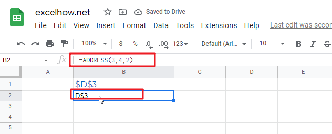
#2 Absolute row, relative column, type the following formula:

=ADDRESS(3,4,2)

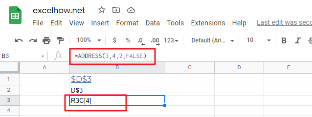
#3 Absolute row, relative column in R1C1 reference style, type the following formula:

=ADDRESS(3,4,2,FALSE)