This post will guide you how to use Google Sheets INT function with syntax and examples.
Table of Contents
Description
The Google Sheets INT function returns the integer portion of a given number. And it will round a given number down to the nearest integer. And the INT function rounds down, so if you provide a negative number, the returned value will become more negative. It means that it will return the first negative number that is less than or equal to the original number. Such as, INT(-5.9), it will return -6.
The purpose of this function is to get the integer part of a number in google sheets. And its returned value is the integer part of the number.
The INT function is a build-in function in Google Sheets and it is categorized as a MATH function.
Syntax
The syntax of the INT function is as below:
= INT (number)
Where the INT function argument is:
- number –This is a required argument. The real number that you want to round down to an integer.
Google Sheets INT Function Examples
The below examples will show you how to use google sheets INT Function to truncate a given number down to the nearest integer.
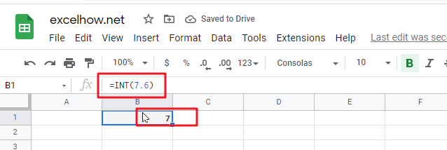
1# get the integer portion of a given number 7.6, enter the following formula in Cell B1.
=INT(7.6)

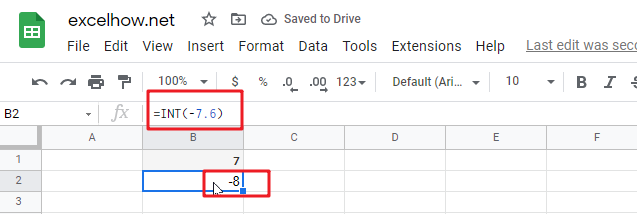
2# rounding a given negative -7.6 down to the nearest integer, enter the following formula in Cell B2.
=INT(-7.6)

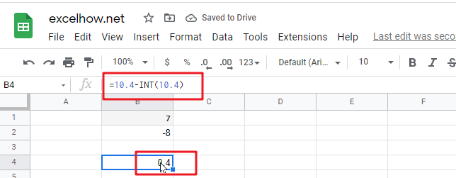
3# get the decimal part of a positive number 10.4, enter the following formula in Cell B3.
=10.4-INT(10.4)
