This post will guide you how to use Google Sheets LOOKUP function with syntax and examples.
Table of Contents
Description
The Google Sheets LOOKUP function looks up a value through a sorted row or column and returns the corresponding value from another row or column.
The LOOKUP function can be used to lookup a value in a one-row or one-column range in google sheets.
The LOOKUP function is a build-in function in Google Sheets and it is categorized as a Lookup function.
Syntax
The syntax of the LOOKUP function is as below:
= LOOKUP (lookup_value, lookup_vector, [result_vector])
Where the LOOKUP function arguments are:
- Lookup_value -This is a required argument. A value that you want to search in the lookup_vector.
- Lookup_vector – This is a required argument. A Range that only contains one row or one column.
- Result_vector – This is an optional argument. A Range that only contains one row or one column. It must be the same size as Lookup_vector. The lookup function will look up the value in the lookup_value range and returns the value from the same position in the result_vector.
Note:
- If
result_vectoris omitted, the Lookup function will return the first column data. - LOOKUP function will only work If data in lookup_vector is sorted. And this function assumes that
lookup_vectoris sorted in ascending order. - When
lookup_valueis not found, LOOKUP function will return the next smallest value in the same row or column. - When
lookup_valueis greater than all values inlookup_vector, LOOKUP function will return the last value. - When
lookup_valueis less than the first value inlookup_vector, LOOKUP function will return the#N/Aerror. - Result_vector must be only a single row or column.
Google Sheets LOOKUP Function Examples
The below examples will show you how to use google sheets LOOKUP Function to search a value from a vector or array.
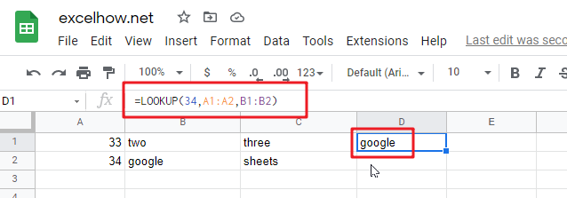
#1 To look up the value “34” in A1:A2 range, then get the value from the same row or column in B1:B2 range, just using the following google sheets formula:
=LOOKUP(34,A1:A2,B1:B2)
