How To Use Google Sheets RATE Function-Free Tutorial

This post will guide you how to use Google Sheets RATE function with syntax and examples in google spreadsheet .

Table of Contents

Description

The Google Sheets RATE function returns the interest rate per payment period of an annuity.

The RATE function is a build-in function in Google Sheets and it is categorized as a Financial Function.

The syntax of the RATE function is as below:

= RATE(number_of_periods, payment_per_period, present_value, [future_value, end_or_beginning, rate_guess])

Where the RATE function arguments are:

number_of_periods -This is a required argument. The total number of payments periods in an annuity.
payment_per_period – This is a required argument. The amount of the payment made each period.
present_value – This is a required argument. The present value of the payments.
future_value – This is an optional argument. The future value or a cash balance you want to attain after the last payment is made. If fv is omitted, it is assumed to be 0 (zero), that is, the future value of a loan is 0.
end_or_beginning – This is an optional argument. The number 0 (zero) or 1 and indicates when payments are due.

Set type equal to	If payments are due
0 or omitted	At the end of the period
1	At the beginning of the period

Guess – This is an optional argument. An initial guess at the internal rate of return. if it is omitted, and it will be set as 0.1 or 10%.

Note:

Make sure that you are consistent about the units you use for specifying rate and nper. If you make monthly payments on a four-year loan at an annual interest rate of 12 percent, use 12%/12 for rate and 4*12 for number_of_periods. If you make annual payments on the same loan, use 12 percent for rate and 4 for number_of_periods.

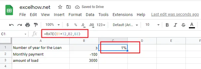
The below examples will show you how to use Google Sheets RATE Function to calculate the interest rate per period of an annuity.

#1 to get the monthly rate of the loan, using the following formula:

=RATE(B1*12,B2,B3)

google sheets rate function1