This post will guide you how to use Google Sheets ROMAN function with syntax and examples.
Table of Contents
Description
The Google Sheets ROMAN function converts a given number to a Roman numeral as text result.
The ROMAN function can be used to format a number in Roman numerals in google sheets. And it’s returned value as a roman numeral in text. And it’s purpose is to convert numbers to Roman numerals.
The ROMAN function is a build-in function in Google Sheets and it is categorized as a Text Function.
Syntax
The syntax of the ROMAN function is as below:
= ROMAN (number, [rule_relaxation])
Where the ROMAN function arguments are:
- Text -This is a required argument. The number to format, between 1 and 3999.
- rule_relaxation -This is an optional argument. The type of Roman numeral that you want to convert. The default form is 0.
Note:
- ROMAN function takes two arguments,
numberandrule_relaxation. The first argument,numbershould be a whole number between 0-3999. And the second argument,rule_relaxationis the degree to which traditional syntax rules may be relaxed. And the default value is zero. And other values are 1-4. - Number should be a positive number between 1 and 3999.
- If number argument is a negative value or out of range (0-3999), and the ROMAN function returns #VALUE! Error message.
Google Sheets ROMAN Function Examples
The below examples will show you how to use google sheets RIGHTB function to extract the rightmost substring from a text string.
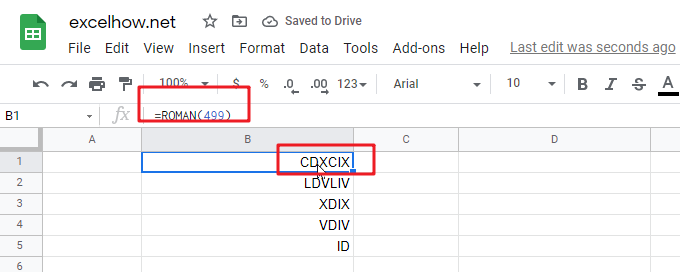
#1 Convert a number 1000 to a Roman numeral, using the following formula:
=ROMAN(1000) //it returns “CDXCIX”

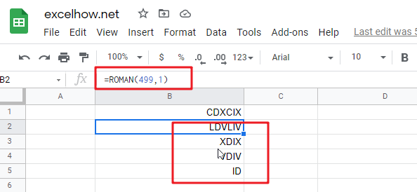
#2 Convert a number 1000 to a Roman numeral with different rule relaxation, using the following formulas:
=ROMAN(1000,1)  //it returns “LDVLIV”
=ROMAN(1000,2)  //it returns “XDIX”
=ROMAN(1000,3)  //it returns “VDIV”
=ROMAN(1000,4)  //it returns “ID”’’

Note: if you want to convert Arabic numbers to Roman number, you can use the ROMAM function. And if you wish convert Roman numbers to Arabic numbers, you can use the ARABIC function in google sheets.