Google Sheets SUBTOTAL Function

This post will guide you how to use Google Sheets SUBTOTAL function with syntax and examples in Google Spreadsheet.

Table of Contents

Description

The Google Sheets SUBTOTAL function returns the subtotal of the numbers in a list or database.

The SUBTOTAL function is a build-in function in Google Sheets and it is categorized as a Math and Trigonometry Function.

The syntax of the SUBTOTAL function is as below:

= SUBTOTAL(function_num, ref1, [ref2])

Where the SUBTOTAL function argument is:

Function_num – This is a required argument. It can be set as 1-11 or 101-111 for the subtotal. 1-11 that includes hidden rows and 101-111 excludes hidden rows.

Function_num (includes hidden values)	Function_num (ignores hidden values)	Function
1	101	AVERAGE
2	102	COUNT
3	103	COUNTA
4	104	MAX
5	105	MIN
6	106	PRODUCT
7	107	STDEV
8	108	STDEVP
9	109	SUM
10	110	VAR
11	111	VARP

Ref1– This is a required argument. The first named range or reference that you want to subtotal.

the below examples will show you how to use Google Sheets SUBTOTAL function to return the subtotal of the numbers in a list.

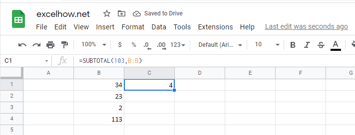
#1 =SUBTOTAL(103,B:B)

google sheets SUBTOTAL Function1

Note: the above formula will call COUNTA function to count the number of cells(B:B) that contain numbers. It will return value 5.

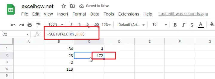
#2 =SUBTOTAL(109,B:B)

google sheets SUBTOTAL Function2

Note: the above Google Sheets formula will call SUM function to add all numbers in range cell B:B, so it will return value: 160.