This post will guide you how highlight rows if the dates in cells have passed from now in your worksheet. How do I highlight rows if dates have passed with the Conditional Formatting feature in excel.
Table of Contents
1. Highlight Rows If Dates Have Passed
Assuming that you have a worksheet that have a bunch of columns and each row has a date column. If the date in the date column goes past from now on and you want to highlight the entire row with red color. How to achieve it. And you need to use the Conditional Formatting feature to highlight all rows that if the dates have passed from now on.
So you need to do the following steps:
#1 select the table that you want to highlight rows if the dates have passed.
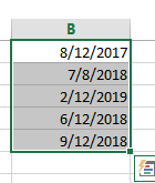
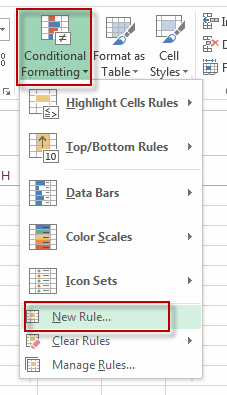
#2 go to HOME tab, click Conditional Formatting command under Styles group, and then click New Rule… from the drop down list. The New Formatting Rule dialog will appear.
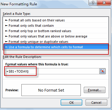
#3 select Use a formula to determine which cells to format in the list box of Select a rule type, and type this formula: =$B1<TODAY() into the text box of the Formula values where this formula is true box.
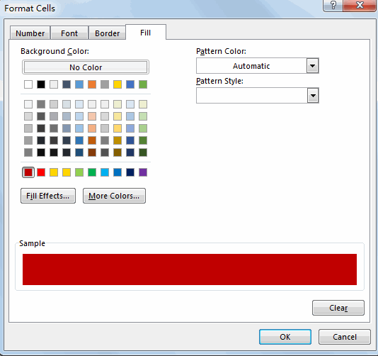
#4 click Format button, switch Fill tab, select the red color, then click OK button.
#5 let’s see the result.
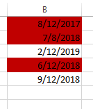
You will see that all rows have been highlighted with red color if the dates have passed from now in your selected range of cells.
2. Video: Highlight Rows If Dates Have Passed
This video tutorial will guide you how highlight rows if the dates in cells have passed from now in your worksheet in Excel 2013/2016/2019.
Leave a Reply
You must be logged in to post a comment.