This post will guide you how to apply shading to every other row or column in Excel. How do I shade every other row in Microsoft Excel 2013/2016.

Shade Every Other Row

---

If you want to share every other row in your current worksheet, you can use a simple conditional formatting formula. Just do the following steps:

Step1: select the range of cells that you want to shade every other row.

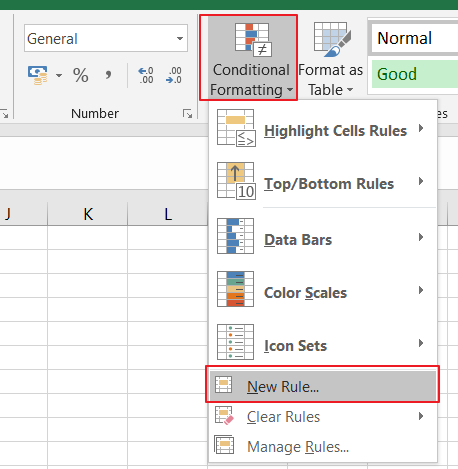
Step2: go to Home tab, click Conditional Formatting command under Styles group, and select New Rule from the dropdown menu list. And the New Formatting Rule dialog will open.

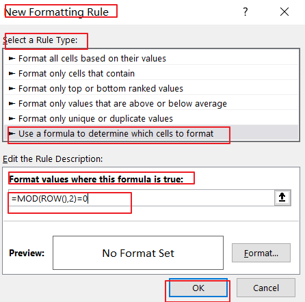
Step3: In the New Formatting Rule dialog box, under Select a Rule Type, click Use a formula to determine which cells to format, and type the following formula into the Format values where this formula is true text box.

=MOD(ROW(),2)=0

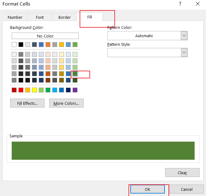
Step3: click Format button, and the Format Cells dialog will open. swith to Fill tab in the Format Cells dialog box, and Select the background or pattern color that you want to use for the shaded rows. click Ok button to back to New Formatting Rule dialog box.

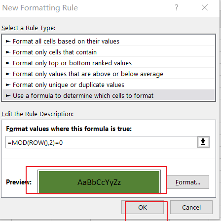
Step4: click OK button, let’ see the last result: