In Excel there are a lot of built-in functions, and AVERAGE is one of the most frequently used functions. In daily work, we may apply AVERAGE function together with some other functions to get average based on some conditions. In this article, we will let you know the method to apply AVERAGE function together with OFFSET function and COUNT function to get the average of last N values in multiple columns.

In this article, we will introduce you the syntax, arguments, and basic usage of above three functions. We will also explain how the formula works with these functions.

EXAMPLE

In this case, we want to calculate the average of last 3 numbers in Row2. The most simple way, we can directly create formula “=AVERAGE(C2:E2)” to get the average as we are already clear that the last values are from range C2:E2. If we want to create a general formula that can cover “returns the average of last N value from multiple columns”, obviously the simple formula with only AVERAGE function cannot meet our demands.

To get the average of last N values for a dynamic range with multiple columns, we can apply AVERAGE function together with other functions to help us. In this article, we also apply OFFSET function together with COUNT function to help us.

FORMULA with AVERAGE & OFFSET & COUNT FUNCTIONS

In E2, enter the formula =AVERAGE(OFFSET(A2,0,COUNT(A2:E2)-3,1,3)), then press Enter, average of last three numbers is 40.

(20+60+40)/3=40, the formula works correctly.

FUNCTION INTRODUCTION

AVERAGE function returns the average of numbers from a given range reference.

Syntax:

=AVERAGE(number1, [number2], …)

Usage:

OFFSET returns a number or a dynamic range based on given five parameters: starting point, row offset, column offset, height in rows and width in rows.

Syntax:

=OFFSET(reference, rows, cols, [height], [width])

Usage 1:

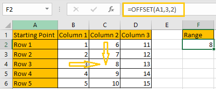
Reference: A1, it is the starting point

Rows: 3, 3 rows below the starting point

Cols: 2, 2 columns to offset to the right of the starting point

Height & Width: optional, no value

Usage 2:

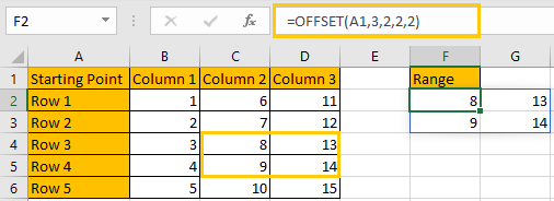
Reference: A1, it is the starting point

Rows: 3, 3 rows below the starting point

Cols: 2, 2 columns to offset to the right of the starting point

Height: 2, it is used together with width, determine the size of the returned range reference, in this case is 2*2 (two rows*two columns)

Width: 2, it is used together with height, determine the size of the returned range reference, in this case is 2*2 (two rows*two columns)

 

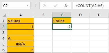
COUNT returns the count of numbers from a given range.

Syntax:

=COUNT(value1, [value2], …)

Usage:

EXPLANATION

=AVERAGE(OFFSET(A2,0,COUNT(A2:E2)-3,1,3))

In this case, COUNT(A2:E2) returns 5, there are five cells with numbers in range reference A2:E2.

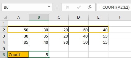
For OFFSET function in this case, the five inputs are:

Reference: A2. It is the starting point in row2.

Rows: 0. That means 0 row below the starting point. It determines the returned range reference is started in row2.

Cols: (COUNT(A2:E2)-3). Returned value is 2, that means 2 columns to offset to the starting point.

Based on above “Reference”, “Rows” and “Cols”, we can confirm the returned range is still stayed in row2, and two columns to offset to A2, so the first column for this range is C column, and the starting cell is C2.

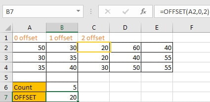
Let’s verify if out thought is correct. Enter =OFFSET(A2,0,2) in B7, then press Enter, formula returns C2 value 20, see screenshot below.

Height: 1. It determines that the returned range is 1-row in height. We stayed in row2 as there is only 1-row in height.

Width: 3. It determines that the returned range is 3-columns in width. From C2, the returned range is expanded from C column to E column, total 3 columns.

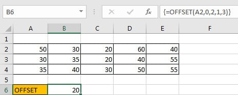
 Based on above “Height” and “Width”, we can confirm the returned range is C2:E2. Enter =OFFSET(A2,0,2,1,3) into B6. As it is an array formula, so press Ctrl+Shift+Enter to get result.

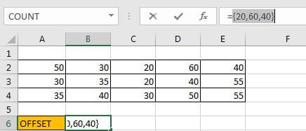
Select {=OFFSET(A2,0,2,1,3)} in formula bar and press F9, {20,60,40} is displayed. {20,60,40} are the values in C2:E2.

Now, =AVERAGE(OFFSET(A2,0,COUNT(A2:E2)-3,1,3)) is equal to =AVERAGE(C2:E2).

Let’s see how the formula works step by step:

Step 1:

Step 2:

Step 3:

Step 4:

Above all, to get average from last N number in multiple columns, we can use below formula:

=AVERAGE(OFFSET(Starting Point,0,COUNT(Range)-N,1,N))

SUMMARY

1. AVERAGE function is used for returning the average of some numbers from a given range in Excel.

2. OFFSET function returns a number or a dynamic range based on given five inputs. Actually, rows, cols, height and width can be input negative numbers.

3. COUNT function only returns count of numbers.

Related Functions

---

• Excel AVERAGE function
  The Excel AVERAGE function returns the average of the numbers that you provided.The syntax of the AVERAGE function is as below:=AVERAGE (number1,[number2],…)….
• Excel COUNT function
  The Excel COUNT function counts the number of cells that contain numbers, and counts numbers within the list of arguments. It returns a numeric value that indicate the number of cells that contain numbers in a range…