In daily work we often need to calculate the average of some numbers based on given conditions or criteria. To calculate average with criteria, we can apply AVERAGEIF of AVERAGEIFS function. AVERAGEIFS function can handle more than one group of criteria range and criteria. In this article, we will show you how to calculate average of numbers whose corresponding cells in another group are not blank. Thus, we need to know some knowledge of AVERAGEIFS function.

In this article, we will let you know the syntax, arguments, and basic usage about AVERAGEIFS function, and apply it to build a formula, also let you know the calculation steps of the formula.

1. EXAMPLE

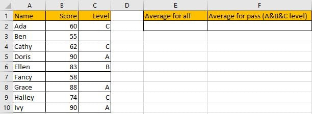
Refer to “Score” column, some numbers are listed in range B2:B10. “Level” column is used for providing a level based on scores. In E2 and F2, we calculate the average of all scores and qualified scores separately. To calculate average of all scores, we can directly use AVERAGE function. To calculate average of qualified scores (cell is not blank in Level group), we need to add criteria to filter them, we can apply AVERAGEIFS function, it is also one of the most common used functions in Excel.

First, In C2, enter “=AVERAGE(Score)”. Then press Enter, AVERAGE function returns 73.33333333.

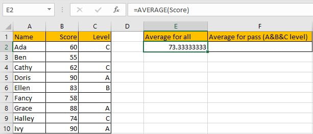
You can adjust decimal places by “Increase Decimal” or “Decrease Decimal” in “Number” section.

Keep clicking on “Decrease Decimal” button till decimal places is ok for you. Keep two decimal places in this case.

Now we can apply AVERGAEIFS function to calculate the average of qualified scores.

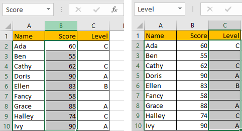
Before creating the formula, name range “B2:B10” to “Score”, “C2:C10” to “Level” in Name Box.

2. CREATE A FORMULA with AVERAGEIF FUNCTION

Step 1: In F2, enter the formula:

 =AVERAGEIFS(Score,Level,"<>").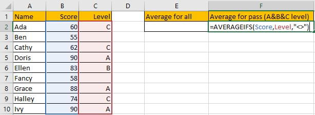

Step 2: Press Enter after typing the formula.

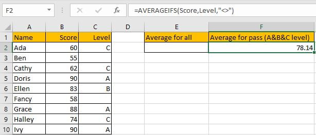
Only B2, B4, B5, B6, B8, B9 and B10 meet our given criteria “level is A or B or C”, so we calculate the average of numbers in above cells, total 7 numbers. (60+62+90+83+88+74+90)/7=78.14285714, keep two decimal places 78.14. The formula works correctly.

a. FUNCTION INTRODUCTION

AVERAGEIFS function is AVERAGE+IFS. It returns the average of some numbers in a range based on one or more given conditions or criteria.

Syntax:

=AVERAGEIFS(average_range, criteria_range1, criteria1, [criteria_range2], [criteria2],…)

It supports wildcards like asterisk ‘*’ and question mark ‘?’, also supports logical expressions like ‘>=’,’<=’. If wildcards or logical operators are required to build criteria, they should be enclosed into double quotes (““). In this case we entered “<>” to represent criteria.

b. EXPLANATION

After expanding values, the formula is displayed as:

=AVERAGEIFS({60;55;62;90;83;58;88;74;90},{"C";0;"C";"A";"B";0;"A";"C";"A"},"<>")

Note: 0 is recorded in this array to represent blank cells.

In the formula, the criteria is “<>” (“not equals to” operator), based on this criteria, cells without any level in “Level” column cannot meet our condition, so for the corresponding values in the average range, they are excluded in calculation.

{60;55;62;90;83;58;88;74;90} -> {60;0;62;90;83;0;88;74;90} – Ignore blank cells

Now this new array only contains numbers. We can calculate the average now (60+62+90+83+88+74+90)/7=78.14.

3. Related Functions

• Excel AVERAGE function
  The Excel AVERAGE function returns the average of the numbers that you provided.The syntax of the AVERAGE function is as below:=AVERAGE (number1,[number2],…)….
• Excel AVERAGEIF function
  The Excel AVERAGEAIF function returns the average of all numbers in a range of cells that meet a given criteria.The syntax of the AVERAGEIF function is as below:= AVERAGEIF (range, criteria, [average_range])….
• Excel AVERAGEIFS function
  The Excel AVERAGEAIFS function returns the average of all numbers in a range of cells that meet multiple criteria.The syntax of the AVERAGEIFS function is as below:= AVERAGEIFS (average_range, criteria_range1, criteria1, [criteria_range2, criteria2],…)….