Sometimes we need to calculate the average for a list or a range of numbers, but blank cells and zero cells may be also included in the selected range, so if these invalid cells are included, we often get error when calculating the average.

This post will guide you on how to calculate average while ignoring blank and zero cells in Excel. By default, Excel’s AVERAGE function includes all cells in the specified range, including blank cells and cells that contain zero values. However, you can use formulas such as AVERAGEIF or AVERAGEIFS to exclude these cells from the calculation.

1. Video: Calculate Average Ignore Blank and Zero Cells in Excel

In this video, you’ll learn how to use the AVERAGEIF formula to calculate the average while ignoring blank or zero cells in Excel.

2. Average Cells in Excel

If you only want to average a range of cell in Excel, and you can use the AVERAGE function. Just type the following formula:

=AVERAGE(A1:C5)

This formula will calculate the average of all the cells in the given range, including  blank cells and cells that contain zero values.

3. Calculate Average Ignore Blank and Zero Cells by Formula

Precondition:

Prepare below table. There are some zero cells and blank cells. We will ignore them when calculating the average.

This is the most convenient way to calculate the average for selected range without zero and blank cells. You can use the AVERAGEIF function with a criteria that excludes blank and zero cells. Just do the following steps:

Step 1: Select a blank cell where you want to display the last average result, for example E2.

Step2: Enter the following formula in the formula bar.

 =AVERAGEIF(A1:C5,"<>0").

Step 3: Press Enter to get the average. Verify that average is calculated properly.

This formula will exclude blank cells and cells that contain a zero value from the calculation.

4. Calculate Average Ignore Blank Only

Excel can calculate the average ignore the blank cells automatically. Zero numbers are still included. You can use the AVERAGEIF function with the criteria “<>” or AVERAGE function only to exclude blank cells.

Type one of the below formula in a blank cell where you want to display the average result:

=AVERAGE(A1:C5)

Or

=AVERAGEIF(A1:C5,"<>")

You may think if we remove all zero values and left them as blank cells, then we can use AVERAGE function directly without other index or parameter. Well, if you remove them totally, you can apply AVERAGE function directly, but, if you just make these zero numbers invisible in the table, you may get improper value by formula.

See example below:

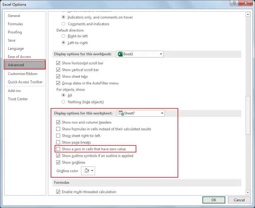
Step1: Click File (it is adjacent to Home) in the ribbon, then select Options to enter Excel Options window.

Step2: On Excel Options window, in the left panel, click Advanced, then drag the scrollbar to the middle, under Display options for this worksheet, uncheck ‘Show a zero in cells that have zero value’ option. Then click OK.

Step3: Then you will find that zero value is ‘removed’ from your table. Only blank cells exist now.

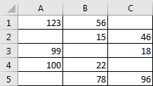
Step4: In E2 enter the formula =AVERAGE(A1:C5). Then press Enter to check the result.

See, we still get the average with zero included. So, you cannot apply AVERAGE function without zero cells by disable showing them in the table.

5. Ignore or Hide Blank Cells in Excel Pivot Table

You can also filter out the blank cells or rows in a pivot table by using the filter options.

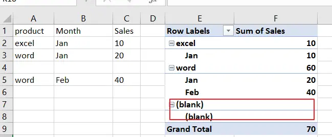
You just need to click on the drop-down arrow next to the column or row header that you want to filter, and then uncheck the “(blank)” option in the filter menu.

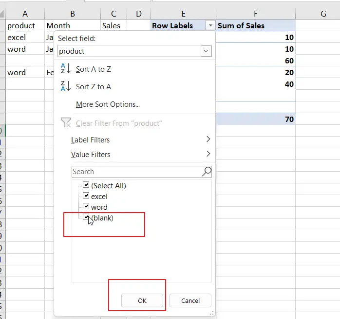
This will hide all the cells or rows that have blank values in that field.

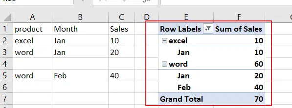
If you want to filter out multiple columns or rows, you can use the “Filter” or ” Insert Slicer” buttons on the ribbon to apply more advanced filters to your pivot table.

6. Conclusion

In your daily work, excluding blank and zero cells when calculating averages is an very useful task that can save you time and provide more accurate results by the above steps in my article.

Just enjoy it.