If you need to calculate the sum of a column in Excel while ignoring #NA errors, this post will guide you through three different methods to accomplish this task. Each method has its own advantages and limitations, so you can choose the one that works best for your specific situation.

Additionally, if you prefer to use VBA code to automate this process, we will provide you with an example that uses the Application.InputBox function to select the range of cells to sum and the destination cell for the result.

1. Video: Sum a Column of Cells Ignore #N/A

This video will demonstrate three methods, including formulas and VBA code, for calculating the sum of a column in Excel while ignoring #NA errors.

2. Sum a Column of Cells Ignore #N/A Using SUMIF Function

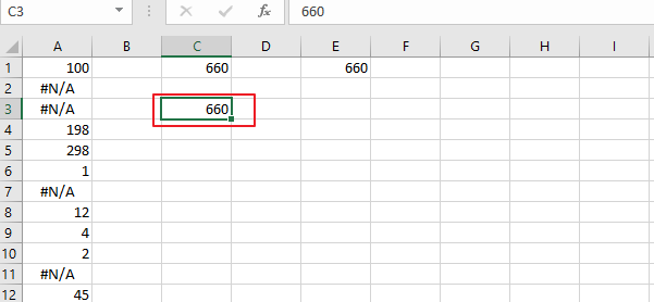
To Sum a column of cells while ignoring #N/A errors in Excel, you can use the SUMIF function. Here’s how you can do it:

Step1: in an empty cell, type the following SUMIF formula:

=SUMIF(A1:A12,"<>#N/A")

Note: Assuming that the cells you want to sum are in the range A1:A2.

Step2: press Enter key in your keyboard.

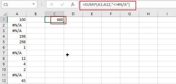
This formula uses the SUMIF function to sum only the cells in the specified range that are not equal to “#N/A“.

3. Sum a Column of Cells Ignore #N/A Using SUM Array Formula

You can also use another formula to sum a column of cells ignore #N/A error based on the SUM function. Here is the formula:

=SUM(IF(ISNUMBER(A1:A12),A1:A12,0))

In a blank cell, type this formula, then Press Ctrl+Shift+Enter to enter the formula as an array formula.

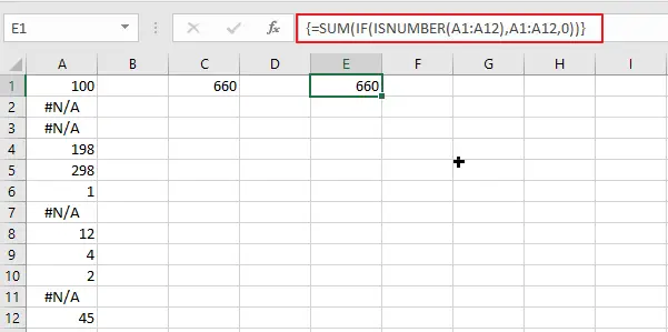
This formula uses the SUM function with an array formula to sum only the cells in the specified range that are numbers. Any #N/A errors are treated as non-numeric and are converted to zero by the IF function.

4. Sum a Column of Cells Ignore #N/A with VBA code

If you want to quickly sum a column of cells or a selected range of cells while ignoring #N/A errors in Excel, you can also use an VBA code to achieve it. Just do the following steps:

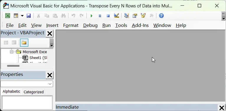
Step1: pressing Alt+F11 shortcut to open the Visual Basic Editor in Excel

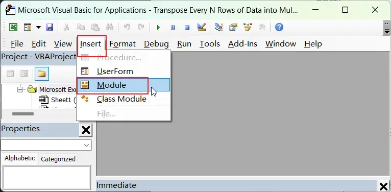
Step2:  click Insert menu to insert a new module named “Module1”

Step3:  paste the code into the module.

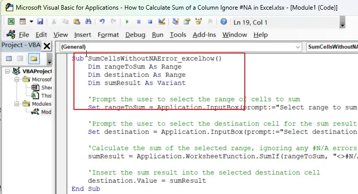
Sub SumCellsWithoutNAError_excelhow()
    Dim rangeToSum As Range
    Dim destination As Range
    Dim sumResult As Variant
    
    'Prompt the user to select the range of cells to sum
    Set rangeToSum = Application.InputBox(prompt:="Select range to sum (ignoring #N/A errors):", Type:=8)
    
    'Prompt the user to select the destination cell for the sum result
    Set destination = Application.InputBox(prompt:="Select destination cell for sum result:", Type:=8)
    
    'Calculate the sum of the selected range, ignoring any #N/A errors
    sumResult = Application.WorksheetFunction.SumIf(rangeToSum, "<>#N/A")
    
    'Insert the sum result into the selected destination cell
    destination.Value = sumResult
End Sub

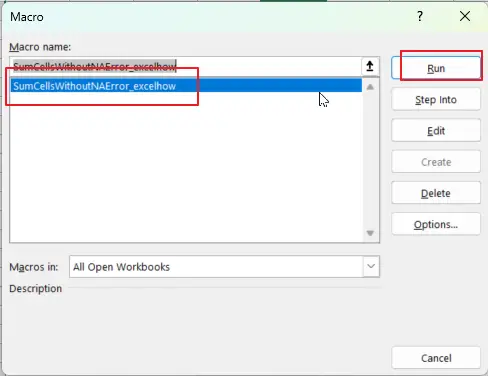
Step4:  Press ALT + F8 to open the Macro dialog box. Then select the macro named “SumCellsWithoutNAError_excelhow” from the Macros list.

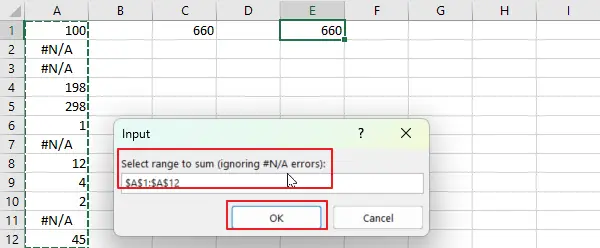
Step5:  select the range of cells to sum in your current worksheet.

Step6: select the destination cell for the sum result.

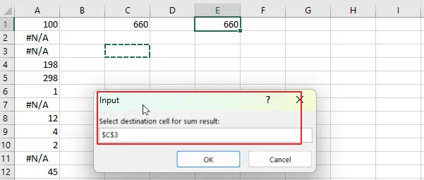
Step7: The macro will then calculate the sum of the selected range, ignoring any #N/A errors, and insert the result into the selected destination cell.

5. Related Functions

• Excel SUMIF Function
  The Excel SUMIF function sum the numbers in the range of cells that meet a single criteria that you specify. The syntax of the SUMIF function is as below:=SUMIF (range, criteria, [sum_range])…