This post will guide you how to change the border color of selected cells in your worksheet in Excel 2013/2016. How do I change border colors to multiple sections of your worksheet in Excel.

• Change Cell Border Color with Border Command
• Change Cell Border Color with Font Setting

Change Cell Border Color with Border Command

---

Assuming that you have a list of data in range A1:B6, and you want to change the border color of this range from the default gray color to red color in your current worksheet, just do the following steps:

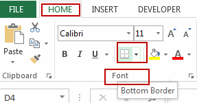
#1 go to HOME tab, click Border command under Font group.

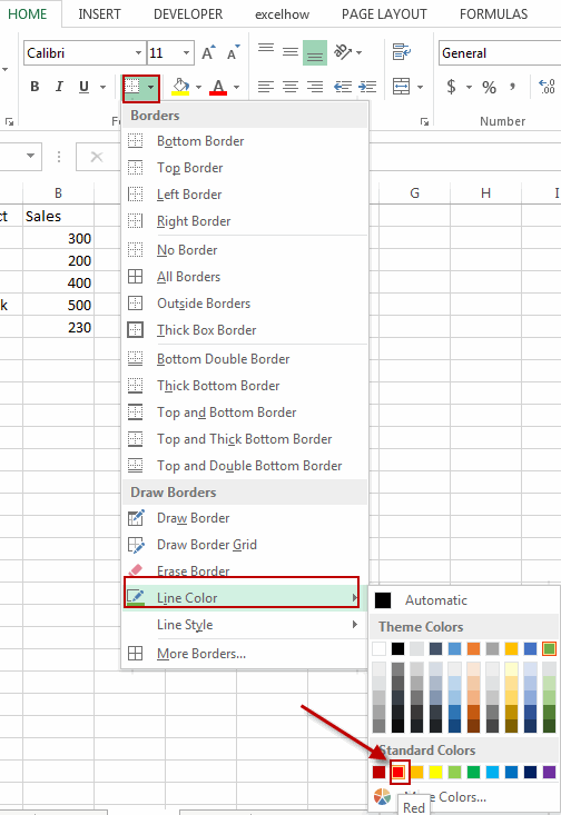
#2 move your mouse over the Line Color menu from the drop down menu list, and select red color from the Color setting box.

#3 you should notice that the current cursor has been changed as a pencil icon. You should drag the pencil cursor from Cell A1 to Cell B6. Then the border color of the range A1:B6 will be changed as red color.

Change Cell Border Color with Font Setting

---

You can change the border color for the different cells or range to organize or sort data so that the data can be easy to read and understand. There is another method to change your border color to distinguish between two ranges of data and help you better understand the data. Here are the steps:

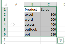
#1 select the cell to which you want to add borders.

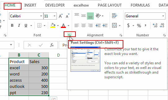
#2 go to HOME tab, click the Font Settings button at the bottom-right corner of the Font group. And the Format Cells dialog will open.

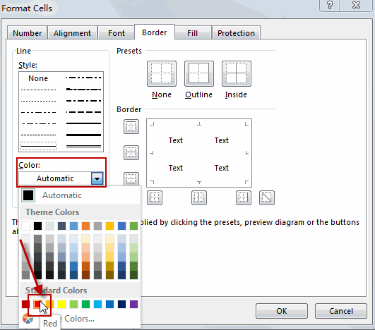
#3 switch to Border tab in the Format Cells dialog box,  and click the drop down menu list of Color , then select one color that you want to use for your borders, such as: red color.

#4 click the Outline button under Presets section, or click the buttons around the border preview at the right of the window to add your borders. Then click Ok button to apply these border settings to your selected range of cells.

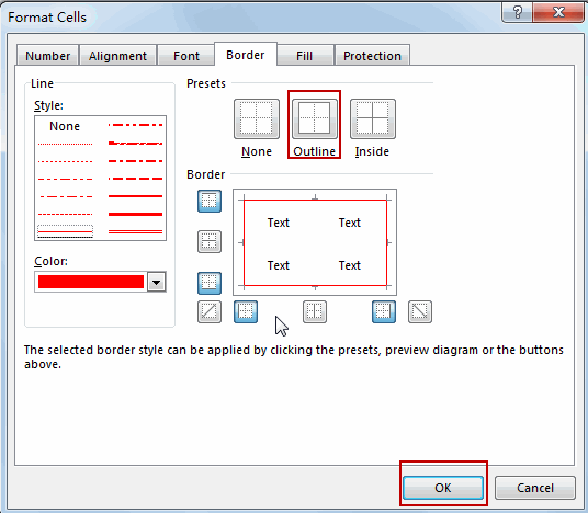
#5 you should notice that the border color of the selected range has been changed as red color.