This post will guide you how to change the font color based on cell value in Excel. How do I color cell based on cell value using the conditional formatting feature in Excel.

1. Changing Font Color Based on Cell Value

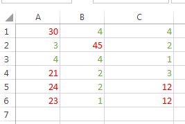
Assuming that you have a list of data in range A1:C6, and you want to change the font color based values in A1:C4 cells, if the value is greater than 5, then changing the font color as red, otherwise, changing the font color as green. To changing the font color based on cell value, you need to do the following steps:

#1 select the range of cells which contain cell values, such as: A1:C6.

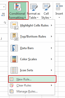
#2 go to HOME tab, click Conditional Formatting command under Styles group, and then click New Rule from the drop down men list. And the New Formatting Rule dialog will open.

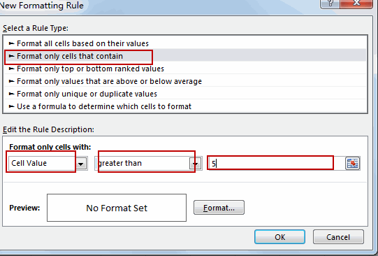
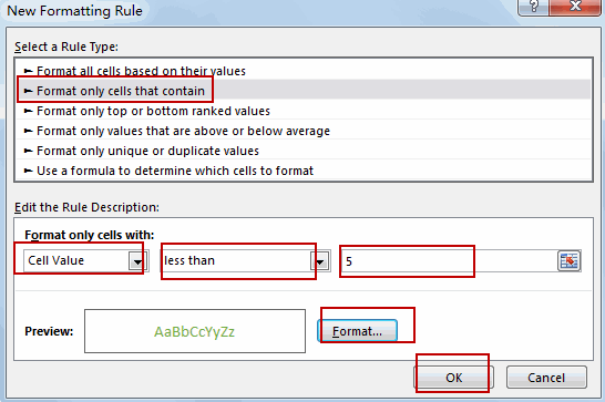
#3 In New Formatting Rule dialog, select Format only cells that contain in the Select a Rule Type list box, chose Cell Value from the first list box, and select greater than from the second list, type number 5 into last text box under Format only cell with section.

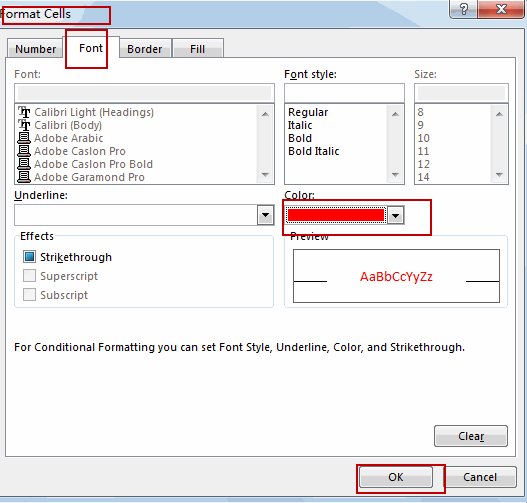
#4 click Format button, and switch to Font tab in Format cells dialog, and choose one color as you need in Color list box. Click OK button.

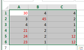
#5 click Ok button. The Font color has been changed as red if the cell value is greater than 5 in the selected range of cells.

#6 repeat step 3, and create a new rule, select less than from the second list , and type number 5 into last text box under Format only cell with section. And click Format button, choose green color in Color list box. And click OK button.

#7  let’s see the last result:

2. Video: Changing Font color Based on Cell Value

This video will demonstrate you how to chagne Fond colore based on Cell value using Conditional formatting feature in Microsoft Excel 2013/2016/2019/365.