Sometimes we need to combine texts in different cells into one cell. It is easy if we use =A1&B1 to combine cells, and we can get proper result if cells have the same cell formatting. But if different formatted numbers, dates or times exist in cells, like content1 in cell A1 is Text, content2 in cell B1 is Date, above formula doesn’t work. If we want to resolve this problem, we can read this article, it will help you to combine cells with different formatting into one cell and at the same time keep their own format properly. It provides two ways to choose, the first one is to strengthen above formula with adding TEXT function, another one is by using Microsoft Word.
Table of Contents
Method 1: Combine Cells with Keeping Cell Formatting by Formula
First, see some examples below.
Example 1: A1-Text & B1-Date

Obviously, formatted date value is changed after combining the two cells. And we cannot change it to previous date in format settings.
Example 2: A2-Text & B2-Number (Percentage)

We can see that value keeps but format is changed. Above all, we need to strengthen the formula by add Text function, details please see below steps.
Step 1: In C1, enter the formula =A1&” “&TEXT(B1,”m/d/yyyy”). Text function can change date, number format to text, so it can display original value in combined cell. For Text function, there are two parameters, one is value, another one is format text, for date, you can also enter mm/dd/yyyy, dddd to display original value.
Step 2: Click Enter and check final result.

Step 3: In C2, enter the formula =A2&” “&TEXT(B2,”0%”). You just need to type number format into Text function to keep B1 original data formatting.

Comment:
You can enter Text Function in Help to check more text formats online.
Method 2: Combine Cells with Keeping Cell Formatting by Microsoft Word
For applying the first method, you need to know the data formatting for all cells. If you don’t know the data formatting, you can choose method 2 to combine cells, see below steps for more details.
Step 1: Copy table from excel to word. Launch word, and create a blank document, then paste copied table on it.

Step 2: Select the table on word document. This is important, otherwise Layout tab below is not displayed.

Step 3: Click Layout tab in Table Tools. There are two “Layout” tabs, make sure you select the proper one.

Step 4: Click Layout->Convert to Text in Data group.

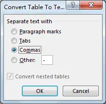
Step 5: Select Commas on Convert Table to Text. Then click OK.

Verify that comma is added between two values. And you may find that texts are combined into one cell.

Step 6: Copy above table and paste it back to excel worksheet.

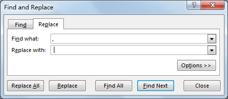
Step 7 (Optional): If you want to remove comma between two data, you can use replace function. Press Ctrl+H to pops up Find and Replace dialog. Enter comma into Find what, space into Replace with, then click Replace All.

Verify that comma is removed.

Comment:
In step 5, if you select Tab as text separator, the two data is still displayed into two cells after pasting it back to excel.