Sometimes we may have so many columns in one worksheet and user cannot view all column headers in one page due to width limit. In this case user has to drag the scrollbar to check the column headers which are located in the columns invisible in current page like column U, column V etc. Is there a convenient way to check column headers directly without drag the scrollbar? This article will help you to resolve this issue by convert column headers to row headers in excel.
Table of Contents
1. Convert Column Headers to Row Headers in Excel
Prepare a table with 10 columns, and the column headers are column 1, column 2… till column 10.

If you want to convert column headers into row headers by a quick way, you can use Paste Special function to implement our requirement. It can transpose a row to a column, in this case column headers saved in row1 can be transposed to specific column properly, and then user can check column headers quickly. Please follow below steps to implement it.
Step 1: Select the range you want to transpose from row to column. In this case if you want to only check the column headers in row for convenient you can only select A1 to J1.
Step 2: Click Ctrl+C to copy this row (the selected range).
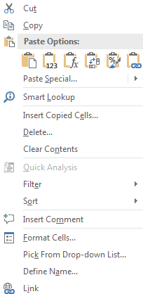
Step 3: In A3 (or other cell you want to paste the column headers), right click to load menu.

Step 4: In Paste Options, select Transpose (T) icon ![]() to implement transpose.
to implement transpose.

Step 5: Check the result. Verify that column headers are listed in one column properly.

This is just a quick way to help you to view all column headers in one column by convenient; if you want all data transpose from row to column (or column to row), you can select all data range to do transpose.
2. Video: Convert Column Headers to Row Headers
This video tutorial we’ll explore the process of converting column headers into row headers. This technique is incredibly useful when you want to restructure your data for better analysis or presentation in Excel.