We have talked that how to count unique numeric values in a data set in Excel in the previous post. And this post will guide you how to count unique numeric values with criteria in the range in Excel 2013/2016 or Excel office 365. How do I count the unique numeric values with a criteria in a list of data with some duplicate values using a formula in Excel. And you can use a formula that uses the SUM function, the FREQUENCY function and the IF function to count unique values in a range based on a criteria in Excel.
Table of Contents
COUNT Unique Numeric Values with Criteria
Assuming you have a list of data range A1:B6 in your worksheet and you wish to count the number of unique score numbers in grade “A” using a formula. And the below introduction will show you the ways to achieve the result. The generic formula is like this:
=SUM(–(FREQUENCY(IF(B2:B7=”A”,A2:A7),A2:A7)>0))
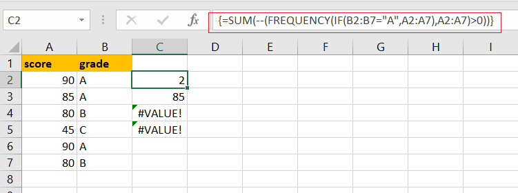
Note: if you are working in Excel 365 version, and you can use a dedicated function called UNIQUE to count unique values. It can be used to count unique values including numeric or text values.
Let’s See How This Formula Works:
=IF(B2:B7=”A”,A2:A7)
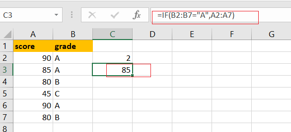
You can use the IF function to filter the value in column B if the grade value in Column B is “A”, then returns the value in Column A. and The result is in an array like this:
{90;85;FALSE;FALSE;90;FALSE}
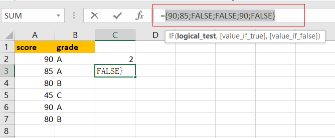
You can notice that if the value is not grade “A”, and it will return the FALSE value. And this array is passed to the FREQUENCY function as the argument.
= FREQUENCY(IF(B2:B7=”A”,A2:A7),A2:A7)
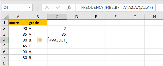
The FREQUENCY function can be used to count each of numeric value in the above array list, and returns an array result, like this:
{2;1;0;0;0;0;0}
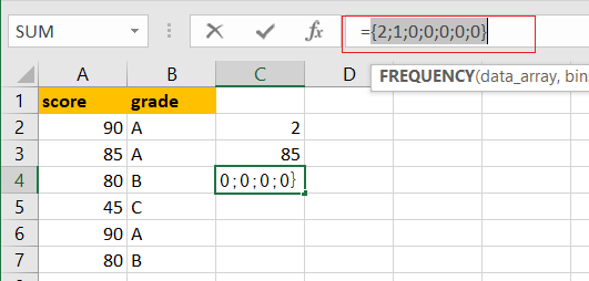
From the above array result, you can see that the FREQUENCY function returns zero for any numbers that appear more that once in the data array, which is why values are zero once a number has been counted.
=FREQUENCY(IF(B2:B7=”A”,A2:A7),A2:A7)>0
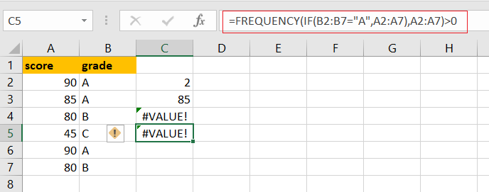
You need to test each values that is greater than zero. The array result is like this:
{TRUE;TRUE;FALSE;FALSE;FALSE;FALSE;FALSE}
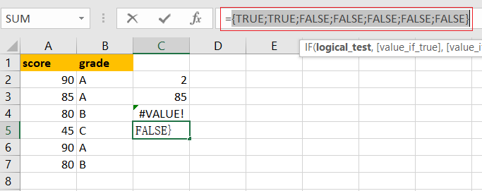
Echo “TRUE” value represents a unique numeric value in the range A2:A7, and you still need to add up the TRUE values with the SUM function.
=–(FREQUENCY(IF(B2:B7=”A”,A2:A7),A2:A7)>0)
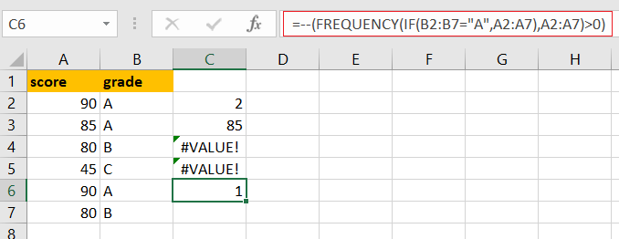
The SUM function can be used to add up logic values in an array, and you need to coerce those values into 1 or 0 by the double negative operator
{1;1;0;0;0;0;0}
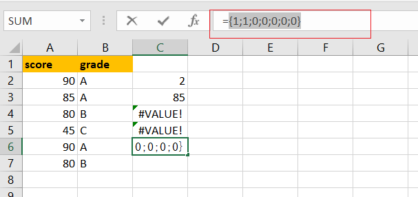
Finally, you can use the SUM function to adds these values up in the above result array and press “CTRL+Shift+Enter” keys to change this normal formula as an array formula, and return the total number is 2.
Related Functions
- Excel SUM function
The Excel SUM function will adds all numbers in a range of cells and returns the sum of these values. You can add individual values, cell references or ranges in excel.The syntax of the SUM function is as below:= SUM(number1,[number2],…)… - Excel FREQUENCY function
TThe Excel FREQUENCY function calculates how often values occur within a range of values. And it will return a vertical array of numbers.The syntax of the FREQUENCY function is as below:= FREQUENCY (data_array, bins_array)… - Excel IF function
The Excel IF function perform a logical test to return one value if the condition is TRUE and return another value if the condition is FALSE. The IF function is a build-in function in Microsoft Excel and it is categorized as a Logical Function.The syntax of the IF function is as below:= IF (condition, [true_value], [false_value])….