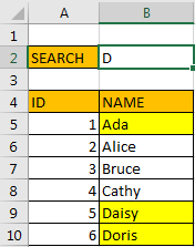
If we entered a value in a cell, and we want to search the whole list to find out all matched values based on the entered value, we can through VLOOKUP function to lookup matched values easily. In another way, we can also create a search box in excel, then use conditional formatting function to mark all matched values in list. This article will introduce you the way to create your own search box in excel, and show you the details to create a new rule in conditional formatting to mark matched values.
Precondition:
Create table like the sample below. We will enter search criteria in B2. Then all matched values in Name list will be marked with proper color.
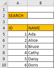
Method: Create A Search Box to Show Matched Values Via Conditional Formatting Function
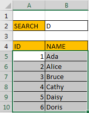
Step 1: Select the whole range of ID and Name lists. Titles are not included.
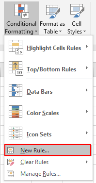
Step 2: Then click Home in ribbon, then click Conditional Formatting in Styles group, select New Rule in menu.
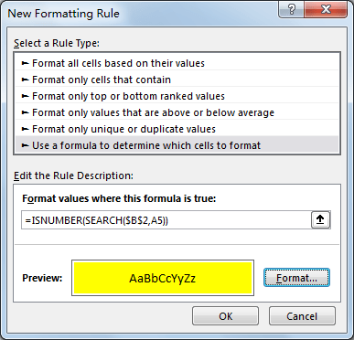
Step 3: On New Formatting Rule dialog, select the last rule type: Use a formula to determine which cells to format.
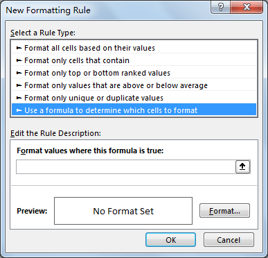
Step 4: In Edit the Rule Description section, in Format values where this formula is true textbox enter the formula =ISNUMBER(SEARCH($B$2,A5)). In this formula, $B$2 is the search box you enter the criteria, A5 is the first cell in your selected range for searching.
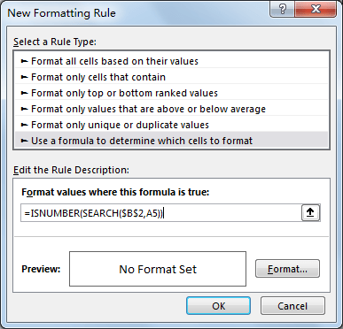
Step 5: Click Format button in Preview section. Verify that Format Cells window is displayed.
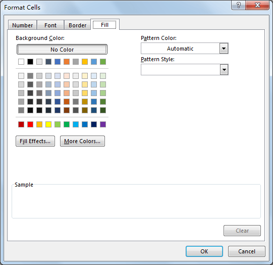
Step 6: Click Fill tab, then select a color as background color. For example, select yellow, then click OK.
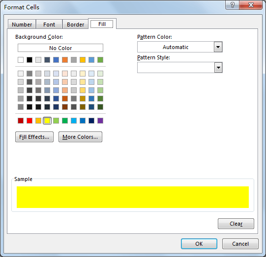
Step 7: After above step, we go back to New Formatting Rule window. You can see that in Preview section, cell is filled with yellow. Click OK.
Step 8: Enter Alice in search box B2. Verify that Alice in list is marked with yellow properly.

Step 9: Only enter D in search box. You can see that Ada, Daisy, Doris are all marked. The searched result is case-insensitive when searching values refer to entered criteria.
