This post will guide you how to display X or Y Axis label in Millions or thousand in Charts in Excel 2013/2016/2019/365. How do I change numbers to Million (M) or Thousand (K) in X Axis label or Y Axis label in Excel Chart. How to Format Axis Label as millions or Thousands in Excel chart.

1. Display Axis Label in Millions or Thousand

Assuming that you have a chart in your worksheet and you want to format the Axis unit as Thousands and Millions to improve the readability of your chart. And this also allows you to present cleaner numbers and avoid inundating your audience with overlarge numbers. To show your numbers in Thousands or Millions in Axis label, just do the following steps:

#1 select the axis (X or Y) that you want to format its unit as thousands or Millions.

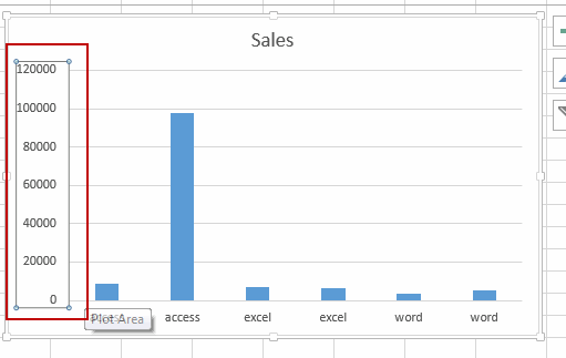
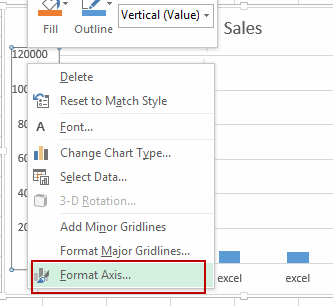
#2 right click on it and select Format Axis from the popup menu list. And the Format Axis pane will display in the right of window.

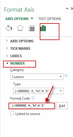
#3 click NUMBER Tab, and type this [>999999] #,,”M”;#,”K” into Format Code text box, and then click Add button.

#4 close the Format Axis pane.

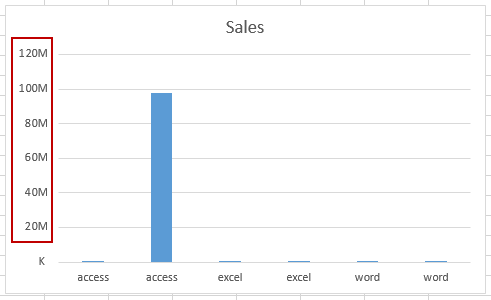
You can see that the selected Axis label has been displayed as thousands (K) or Millions (M).

2. Display Units as Millions or Thousand

If you want to change the display units as millions or thousands in the Axis label, you can also do the following steps:

#1 repeat the above steps 1-2.

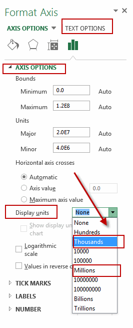
#2 click the Axis Options tab, and then select Millions or Thousands from the Display units dropdown list.

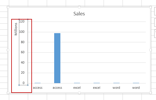
#3 let’s see the result.

3. Video: Display Axis Label in Millions or Thousand

This video will show how to display axis labels in millions (M) or thousands (K) in Excel to simplify data representation in Excel 2013/2016/2019/365.