This post will explain various methods to exclude values from one column based on values in another column in Excel.
Often, while working with large datasets, we need to remove certain values from a column based on criteria from another column. we will cover three different approaches to achieve this: using the VLOOKUP function, the COUNTIF function, and VBA code.
Prepare a table recording the PASS and FAIL status for students. Now we need to exclude students who are listed in PASS column but also listed in FAIL.
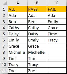
Table of Contents
1. Exclude Values from One Column by VLOOKUP Function
Step1: Insert a new column between column B and column C. Then in C2 enter the formula
=VLOOKUP(B2,$D$2:$D$6,1,FALSE)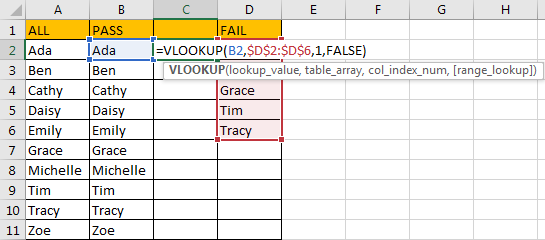
Step2: Click Enter. Verify that Ada is displayed in this cell.
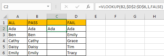
Step3: Drag down the fill handle. Verify that C2:C11 are filled with returned values of VLOOKUP function.
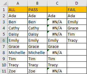
Through the screenshot we can see that values need to be removed are displayed in column C.
Step4: Create a filter on C1. Select row 1, click Data in ribbon, select Filter.
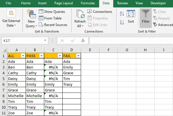
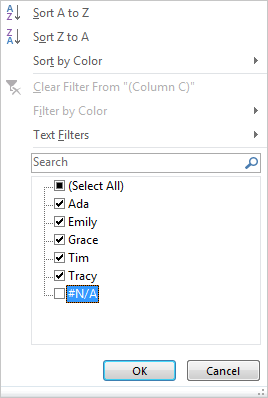
Step5: Click arrow button in C1, then Sort & Filter dialog is displayed. Check on Select All option first (this operation will activate all options checked), then uncheck #N/A. Click OK.
Then values need to be excluded are filtered in column B.
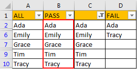
Step6: Now you can highlight them or remove them per your request. If you want to highlight them, just select the range marked in red in above screenshot, and click Home->Fill Color button to highlight them.
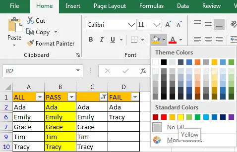
If you want to remove them, just copy this column to another worksheet, and then filter text by color.
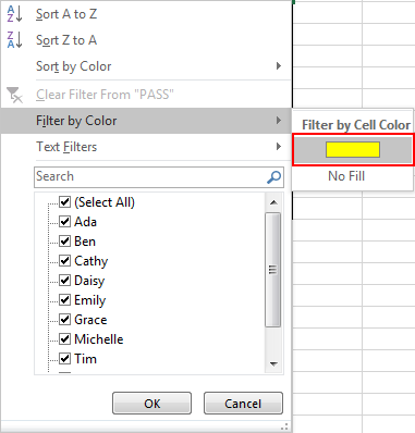
Then delete these filtered cells (press F5 to trigger Go To dialog, and then click Special button, check on Visible cells only option and click OK, all visible cells are selected, then you can delete them). Copy and paste updated column to column B again.
2. Exclude Values from One Column by COUNTIF Function
Steps are similar with VLOOKUP function.
Step1: Insert a new column between column B and column C. Then in C2 enter the formula:
=COUNTIF($D$2:$D$6,B2)COUNTIF function is used for counting how many times B2 appears in range $D$2:$D$6. If B2 value appears in the selected range, COUNTIF returns the times B2 appears, if B2 doesn’t appear, COUNTIF returns 0.
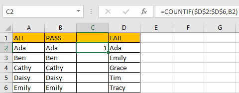
Step2: Drag down the fill handle till reaching the last cell in column C. Verify that C2:C11 are filled with returned value 1 or 0.
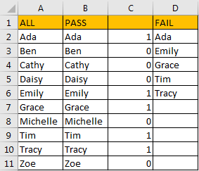
For values in column B, if 1 is displayed in its adjacent cell of column C, this value should be excluded.
Now you can follow step#4-#6 in method1 to exclude them.
3. Exclude Values from One Column Based on Another Column with VBA Code
If you want to exclude values from one column based on values in another column with VBA code, and return an array result, you can use the following steps:
Step1: Open the Excel workbook and press ALT + F11 to open the Visual Basic Editor.
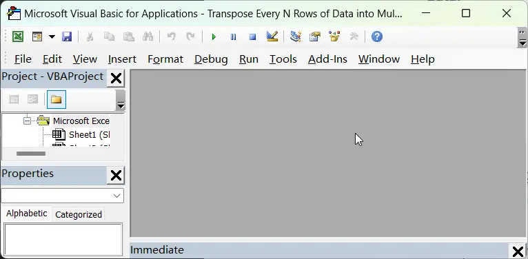
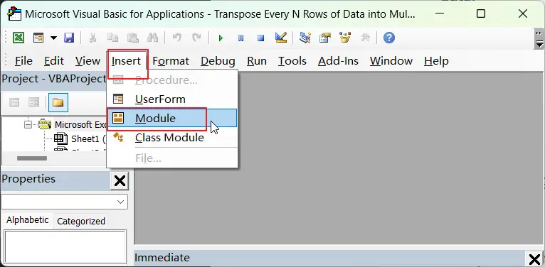
Step2: Click on Insert > Module to add a new module to the workbook.
Step3: Paste the following code into the module. Close the Visual Basic Editor and return to the Excel workbook.
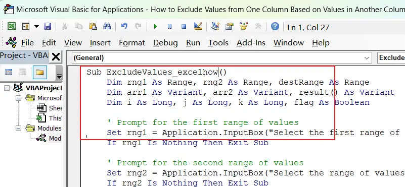
Sub ExcludeValues_excelhow()
    Dim rng1 As Range, rng2 As Range, destRange As Range
    Dim arr1 As Variant, arr2 As Variant, result() As Variant
    Dim i As Long, j As Long, k As Long, flag As Boolean

    ' Prompt for the first range of values
    Set rng1 = Application.InputBox("Select the first range of values to exclude from:", Type:=8)
    If rng1 Is Nothing Then Exit Sub

    ' Prompt for the second range of values
    Set rng2 = Application.InputBox("Select the range of values to exclude based on:", Type:=8)
    If rng2 Is Nothing Then Exit Sub

    ' Prompt for the destination cell
    Set destRange = Application.InputBox("Select the destination cell:", Type:=8)
    If destRange Is Nothing Then Exit Sub

    ' Convert the input ranges to arrays
    arr1 = rng1.Value
    arr2 = rng2.Value

    ' Exclude values based on the second range
    ReDim result(1 To UBound(arr1, 1), 1 To 1)
    For i = 1 To UBound(arr1, 1)
        flag = False
        For j = 1 To UBound(arr2, 1)
            If arr1(i, 1) = arr2(j, 1) Then
                flag = True
                Exit For
            End If
        Next j
        If Not flag Then
            k = k + 1
            result(k, 1) = arr1(i, 1)
        End If
    Next i

    ' Resize the result array
    'ReDim Preserve result(1 To k, 1 To 1)

    ' Write the result to the destination cell
    destRange.Resize(k, 1).Value = result
End Sub
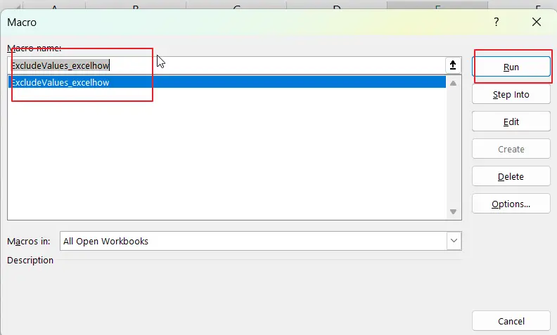
Step4: Press ALT + F8 to open the Macros dialog box. Select the “ExcludeValues_excelhow” macro and click on the “Run” button.
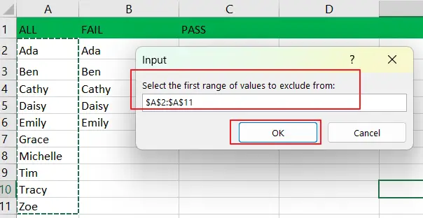
Step5: select the first range of values to exclude from.
Step6: select the range of values to exclude based on.
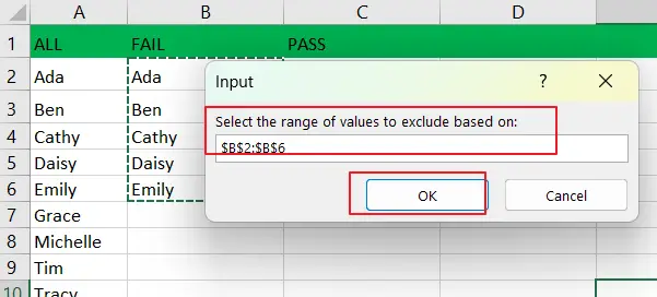
Step7: select the destination cell to place the result.
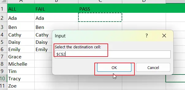
Step8: The macro will exclude the values from the first range based on the values in the second range and write the result to the destination cell.
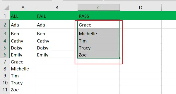
4. Conclusion
Now you should have a clear understanding of how to implement each of these methods and choose the one that suits your needs best.
5. Related Functions
- Excel VLOOKUP function
The Excel VLOOKUP function lookup a value in the first column of the table and return the value in the same row based on index_num position.The syntax of the VLOOKUP function is as below:= VLOOKUP (lookup_value, table_array, column_index_num,[range_lookup])…. - Excel COUNTIF function
The Excel COUNTIF function will count the number of cells in a range that meet a given criteria. This function can be used to count the different kinds of cells with number, date, text values, blank, non-blanks, or containing specific characters.etc.= COUNTIF (range, criteria)…