We can do filter data by some certain criteria for a list or a table in excel. And if the criteria is another list selection in worksheet, how can we filter data from original selected range refer to the new list selection? This article will provide you two methods to filter data based on another list selection by COUNTIF Formula or Advanced Filter Function in excel, you can select one you like to use it in your daily work.
Why we need to learn how to filter data based on another list selection? Actually, we often get a summary (filter range) from others and we just want to get part information by some criteria (criteria range, usually it is another list), see the example below.
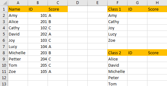
In above table column A, B, C list all students’ Names, IDs and Scores. We want to get ID and Score for class1 and class2 students, we need to filter data from the filter range based on the name list of class1 and class2. Now, you can follow below steps to filter data by different methods.
Table of Contents
Method 1: Filter Data Based on Another List Selection by Formula
Step 1: First, we need to find out which names included in column A also belong to Class1. We can use COUNTIF function to mark these names. In cell D2, enter the formula =COUNTIF($F$2:$F$6, A2). Then click Enter. Verify that we get return value ‘1’ in D2.
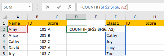

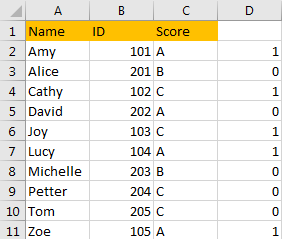
Step 2: Drag the fill handle down to fill all cells. Then we can find that names belong to class1 are marked with number ‘1’.
Step 3: Create a filter on column D. Select on column D, click on Data->Filter, then click dropdown list, only check on number ‘1’, then click OK.
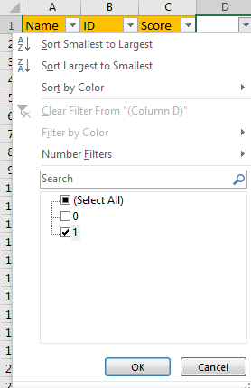
Verify that all names belong to class1 are listed properly with ID and Score.
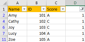
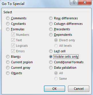
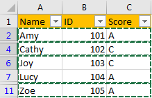
Step 4: Select all filtered data, click F5, on Go To dialog click on Special button, then check on ‘Visible cells only’, then click OK.
Step 5: Copy and paste the selected data to criteria range accordingly.
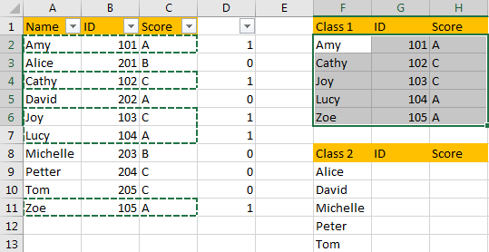
We can repeat above steps to filter data for class2.
Method 2: Filter Data Based on Another List Selection by Advanced Filter
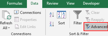
Step 1: Select data you want to do filter, in this case we select A2:C11, select Data->Advanced.
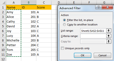
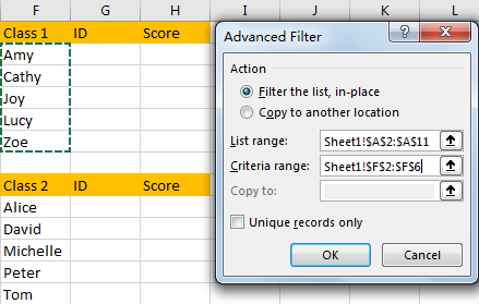
Step 2: On Advanced Filter dialog, check on ‘Filter the list, in-place’, in List range select $A$2:$A$11, in Criteria range, select $F$2:$F$6. Then click OK.
Step 3: After above steps, names are filtered properly.
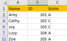
Step 4: Repeat step#4-5 in method 1 to copy and paste filtered data to criteria range.
Related Functions
- Excel COUNTIF function
The Excel COUNTIF function will count the number of cells in a range that meet a given criteria. This function can be used to count the different kinds of cells with number, date, text values, blank, non-blanks, or containing specific characters.etc.= COUNTIF (range, criteria)…