Suppose we have a list of data entry, we want to look up the first positive number among them, is there any way to find it out? And if we want to look up the first or last negative number, how can we do? Actually, to find out the first or last positive/negative number from a list of data, we can apply formula with some functions like INDEX, LOOKUP, MATCH to get them properly. This free tutorial will show you the formulas to help you find out positive or negative number per your request.
Precondition:
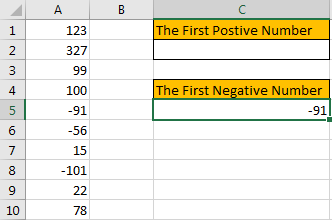
See screenshot below. There are some positive and negative numbers in a column.
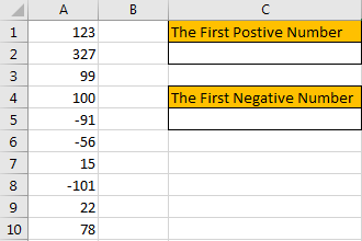
Table of Contents
1. Find the First Positive Number by Formula
Step1: Select a blank cell, enter the formula:
=INDEX(A1:A10,MATCH(TRUE,A1:A10>0,0))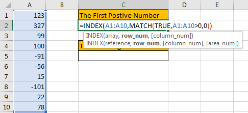
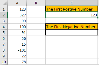
Step2: As it is an array formula, so press Ctrl+Shift+Enter to get result. Verify that the first positive number 123 is displayed properly.
2. Find the First Negative Number by Formula
Step1: Select a blank cell, enter the formula:
=INDEX(A1:A10,MATCH(TRUE,A1:A10<0,0))Just change > in method1 formula to <.
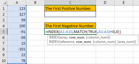
Step 2: As it is an array formula, so press Ctrl + Shift + Enter to get result. Verify that the first negative number -91 is displayed properly.
3. Find the Last Positive Number by Formula
Step1: Select a blank cell, enter the formula:
=LOOKUP(2,1/(A1:A10>0),A1:A10)
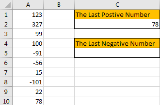
Step2: As it is an array formula, so press Ctrl + Shift + Enter to get result. Verify that the last positive number 78 is displayed properly.
4. Find the Last Negative Number by Formula
Step1: Select a blank cell, enter the formula:
=LOOKUP(2,1/(A1:A10<0),A1:A10)Compare to get the positive number by formula, just change > in the formula to <.

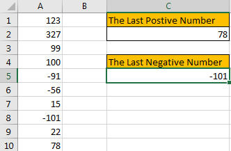
Step2: As it is an array formula, so press Ctrl+Shift+Enter to get result. Verify that the last negative number -101 is displayed properly.
5. Video: Find the First or Last Positive or Negative Number in a Column
In today’s video, we will show you the way to identify the first or last positive or negative number in a list of numbers.
6. Related Functions
- Excel LOOKUP function
The Excel LOOKUP function will search a value in a vector or array.The syntax of the LOOKUP function is as below:= LOOKUP (lookup_value, lookup_vector, [result_vector])…
- Excel INDEX function
The Excel INDEX function returns a value from a table based on the index (row number and column number)The INDEX function is a build-in function in Microsoft Excel and it is categorized as a Lookup and Reference Function.The syntax of the INDEX function is as below:= INDEX (array, row_num,[column_num])… - Excel MATCH function
The Excel MATCH function search a value in an array and returns the position of that item.The MATCH function is a build-in function in Microsoft Excel and it is categorized as a Lookup and Reference Function.The syntax of the MATCH function is as below:= MATCH (lookup_value, lookup_array, [match_type])….