This post will show you how to find the value of the last non-empty cell in a column using XLOOKUP function in Excel 365.

Imagine you’re working on a project where you need to quickly identify the most recent data point in a column. This could be anything from the last sale recorded in a sales log to the final entry in a timesheet. The traditional method of scanning each row individually is not only time-consuming but also prone to human error. Fortunately, Excel offers a smarter way.

The challenge with traditional methods, such as using the VLOOKUP or even a manual search, is that they either require you to scroll through each row or have limitations in handling non-sequential data. But with XLOOKUP, we can automate this process and ensure that we always get the most recent data point, regardless of the presence of empty cells.

Let’s consider a practical scenario. You’re managing a team’s performance data, and you have a spreadsheet with daily updates. The data is dynamic, with new entries being added regularly, and some days might not have any entries at all. Your task is to quickly find the last recorded entry to analyze the team’s most recent performance.

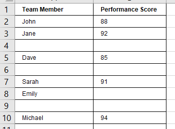
In this table, the “Performance Score” column is what interests us. We want to find the last recorded score without manually searching through each row.

Finding the Last Non-Empty Cell with XLOOKUP

The XLOOKUP function is a versatile tool that can be used to find the last non-empty cell in a column. It’s designed to return the first match by default, but with a slight modification, it can be used to find the last match. Here’s how you can set up the formula:

=XLOOKUP(TRUE,B2:B9<>"",B2:B9,,,-1)

This formula uses the XLOOKUP function to search for the last non-empty cell in the range B2:B9. Here’s a breakdown of how it works:

• B2:B9<>””：This part of the formula creates a logical array where each element is TRUE if the corresponding cell in the range B2:B9 is not empty, and FALSE if it is empty.

• The XLOOKUP function searches for the first TRUE value in the logical array created above. Since we’re looking for the last non-empty cell, the -1 argument tells XLOOKUP to return the last match.

Now, let’s talk about why we chose TRUE as our search value. In XLOOKUP, the search value is the target that the function looks for within the lookup array. By using TRUE, we’re leveraging the fact that TRUE is a logical value that can be compared to the array of TRUE and FALSE values we created. It’s a clever way of harnessing the power of XLOOKUP to find the last non-empty cell.

Moreover, this formula is dynamic. As new data is added to the range or existing data is removed, the formula automatically adjusts to provide the correct result. There’s no need to manually update the range or the formula—it simply works.

Expanding the Example

Now, let’s consider a more complex scenario. Imagine you’re tracking project progress with multiple teams reporting their updates in a shared spreadsheet. You need to find the most recent update from each team.

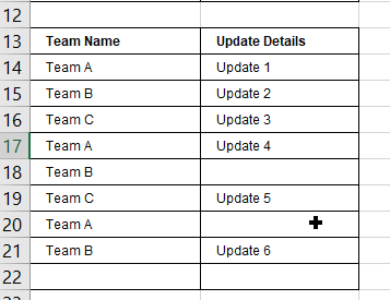
In this table, the “Update Details” column contains the updates from each team. Our goal is to find the value of the last non-empty cell in the “Update Details” column for each team.

=XLOOKUP(1, (A12:A20="Team A")*(B12:B20<>""),B12:B20,,,-1)

This formula will return the most recent update details for Team A. We can copy this formula and adjust the “Team A” part to filter for other teams.

Let’s see how this formula works:

• Logical Array Creation:
  • (A12:A20=”Team A”): This part creates a logical array where each element is TRUE if the corresponding cell in the range A12:A20 is “Team A”.
  • (B12:B20<>””): This part creates another logical array where each element is TRUE if the corresponding cell in the range B12:B20 is not empty.
  • When these two arrays are multiplied together (A12:A20=”Team A”)*(B12:B20<>””), it results in an array where each element is 1 (since TRUE * TRUE = 1) only if both conditions are met (i.e., the cell in column A is “Team A” and the corresponding cell in column B is not empty).
• The first argument 1 is the value we’re looking for in the combined logical array. It corresponds to the rows where both conditions are met.
• The second argument (A12:A20=”Team A”)*(B12:B20<>””) is the array where XLOOKUP will search for the value 1.
• The third argument B12:B20 is the range from which XLOOKUP will return the corresponding value.

The fifth argument -1 tells XLOOKUP to search from the end of the array to the beginning, ensuring it finds the last occurrence of 1 (i.e., the last non-empty cell in column B for “Team A”

Conclusion

And there you have it! With the XLOOKUP function, finding the last non-empty cell in a column is a breeze. This technique is not only efficient but also minimizes the chance of errors, ensuring that your data analysis is accurate and reliable.

Video: Finding the Last Non-Empty Cell with XLOOKUP

We’ll be diving into the use of XLOOKUP function to find the value of the last non-empty cell in a column. Let’s get started!