This post will guide you how to format cells containing #N/A Error in Excel. How do I add conditional formatting to cells that containing #N/A Error in Excel 2013/2016/2019/365.

The #N/A error often occurs when a lookup or reference function cannot find a matching value. By formatting cells with the #N/A error, you can visually identify the missing or invalid data points.

1. Format cells containing #N/A Error

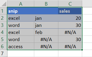
Assuming that you have a range of cells which contain #N/A errors, and you want to use conditional formatting to highlight cells which contain #N/A error. How to do it. Just do the following steps:

As #N/A is not a text, you need to use ISNA function to match on an error of this type in the Conditional Formatting.

Step1: select the range of cells that contain #N/A errors and you want to highlight.

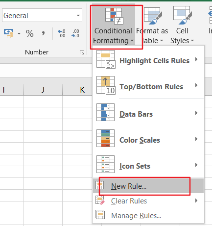
Step2: go to Home Tab, and click Conditional Formatting command under Styles group. Then click New Rule from the popup menu list. And the New Format Rule dialog will open.

Step3: select use a formula to determine which cells to format in the Select a Rule Type list box, and enter the following formula in the text box of Format values where this formula is true:

=ISNA(A1)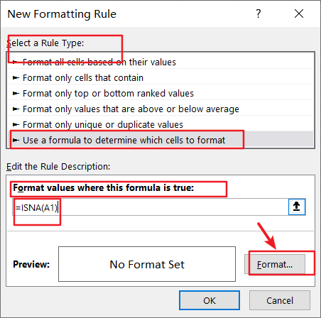

Note: Cell A1 is the first cell that you select.

Step4: click Format button, and the Format Cells dialog will open. Switch to Fill tab in the Format Cells dialog , and choose one color as background color. And click Ok button.

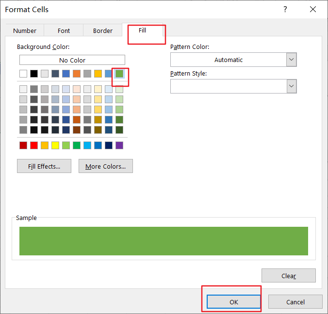
Step5: then returns to the new Formatting Rule dialog box, click Ok button again.

Step6: You would see that all cells which contain #N/A error have been highlighted with green color as you set.

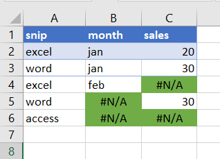
Now, any cells within the selected range that contain the #N/A error will be formatted according to the formatting options you specified in the Format Cells dialog box.

2. Video: Format cells containing #N/A Error

This video will show you how to format cells containing the #N/A error using Conditional formatting feature in Excel.