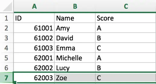
We already know hide and unhide row or columns by right click ‘Hide\Unhide’ in Excel. And there is another way to hide row or columns by Group function, and on the other side unhide row or columns by it as well.
Prepare a table contains ID, Name and Score information. By ID classification we can think that these students can be divided into two groups, ID started from 0610… belongs to group1, and ID started from 0620… belongs to group2.
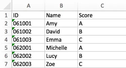
If we want to high group1 or group2, we all know that we can select the rows we want to hide and directly right click and select Hide to hide rows for group. Is there another way to hide them?
Hide Row or Columns by Group Function in Excel
Step 1: Select entire rows you want to hide. In this case we select row5 to row7.

Step 2: Click on Data->Group to group rows.

You can find that after clicking on Group icon, outline area is displayed, and a minus sign is auto displayed in front of the selected rows, actually it displays just before row8. Obviously user can click on the minus sign.

Step 3: Click on the minus sign. Verify that rows are hidden now. And minus sign is change to plus sign.

Step 4: Click on plus sign again, verify that all hidden rows are expanded again.
Notes:
If you have only one single level of group, number 1 and 2 are displayed in outline; if you add a new group within the created group, it will show number 1, 2 and 3 in outline.
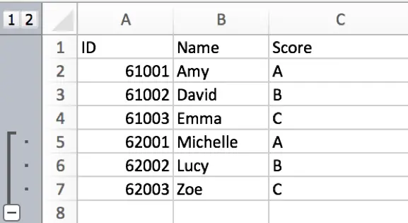
In below screenshot we create a new group only contains two students. Now there two levels of groups.
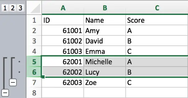
Step 5: If user want to ungroup the group, select the rows you want to ungroup, and click on Data->Ungroup.

For example, after step#4, only select row5 and row6, click Ungroup. Then you can find only row7 is included in group.
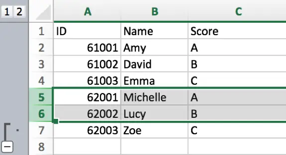
Step 6: Select row7, click on Data->Ungroup->Clear Outline.

Verify that group is removed now. Minus sign or plus sign is cleared.
