Sometimes we want to find all zero value cells in worksheet and hide zero value to make the data to be checked easier. In this article, we will provide you some simple ways like changing format settings or by IF function to hide zero values.
Prepare a table with some 0 value cells.

At the first time, we may feel all values are filled with values to reflect the consumption, but actually 0 value is invalid for statistic, so we can just hide these 0 cells.
Table of Contents
1. Hide 0 in Excel by Format Settings
As number or text format is determined by format settings in Excel, so we just need to change the format for 0 to hide it in Excel.
Step 1: Select the table, and right click your mouse, select Format Cells…. You can also directly click Ctrl+1 to load Format Cells screen.

Step 2: On the pops up Format Cells screen, select Custom under Category List.
Step 3: In Type field, enter 0;-0;;@.
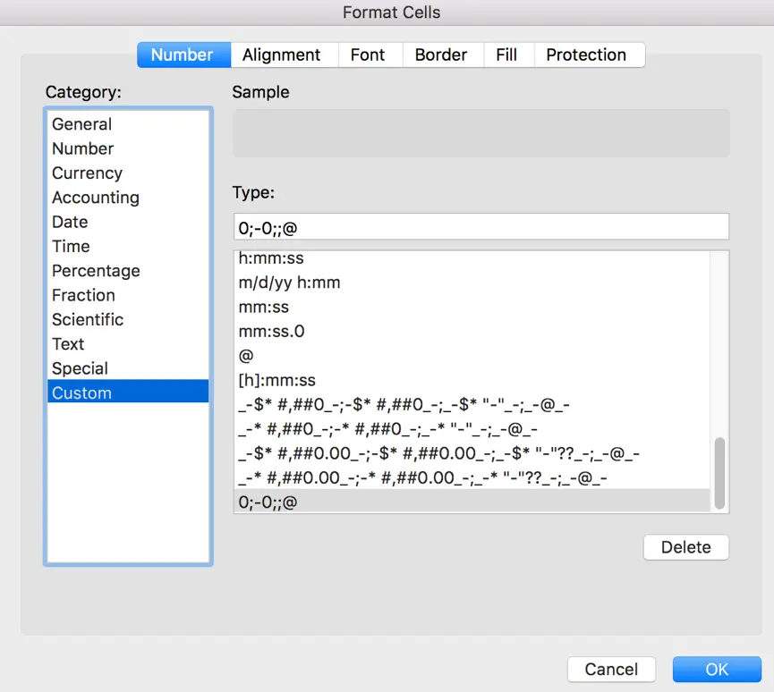
Step 4: The last step, click on OK button to complete above operations. Then you will find all 0 values are hidden in the table.

Notes:
If you want to re-display the hidden 0 values in the table, just repeat above steps and in Format Cells->Customer->Type field select General and click OK.
2. Hide 0 in Excel by Conditional Formatting Feature
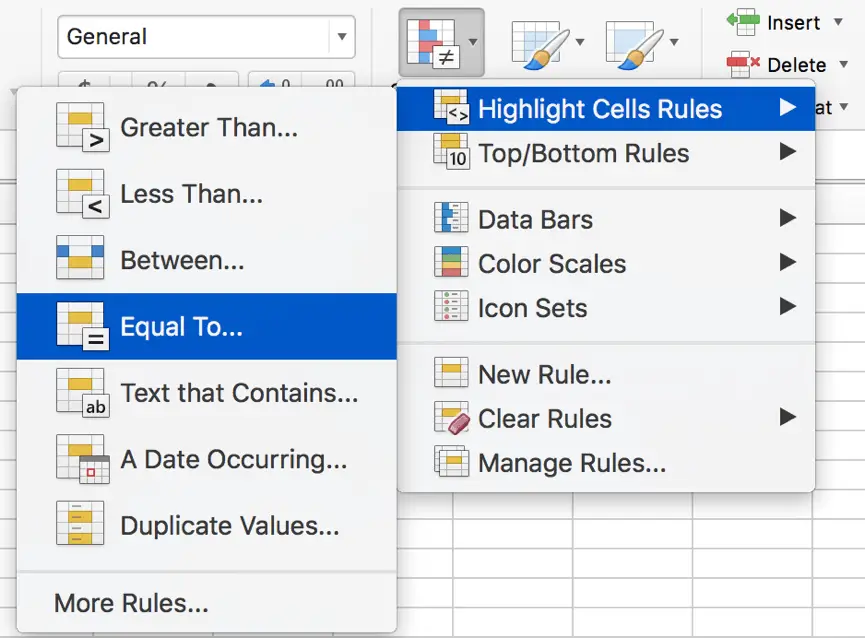
Step 1: Select the table. In Home tab, click the arrow button attach to Conditional Formatting.

Step 2: Select Highlight Cells Rules->Equal to….
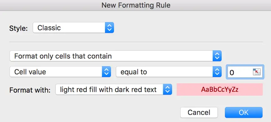
Step 3: In New Formatting Rule screen, enter 0 in the left textbox.
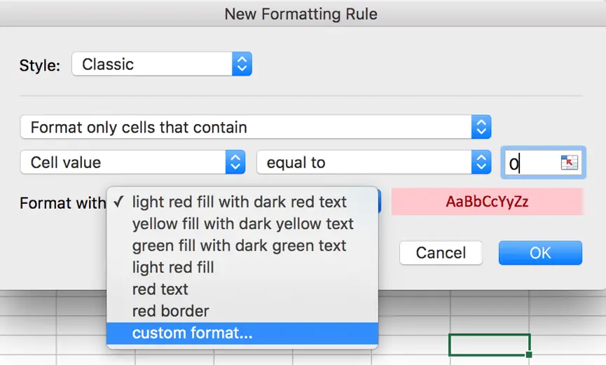
Step 4: In Format with: field, click on the arrow button, and select custom format….
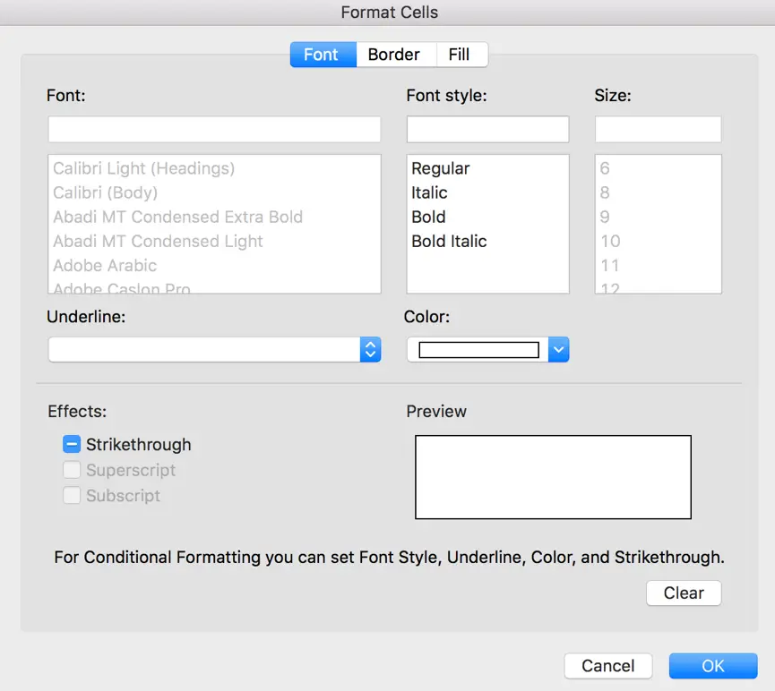
Step 5: In the pops up Format Cells screen, click on Font, change font color from default settings to white.
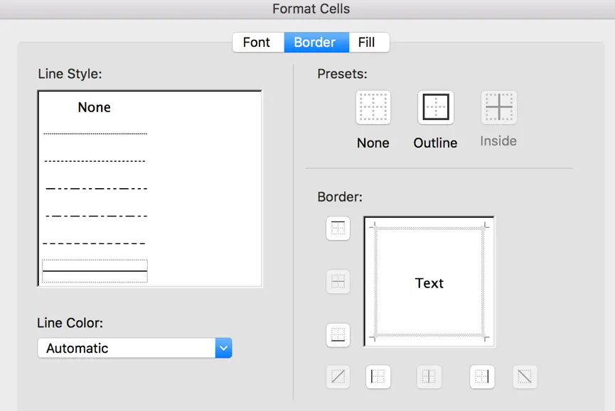
Step 6: Click on Border, and keep Line Color as Automatic as below settings.
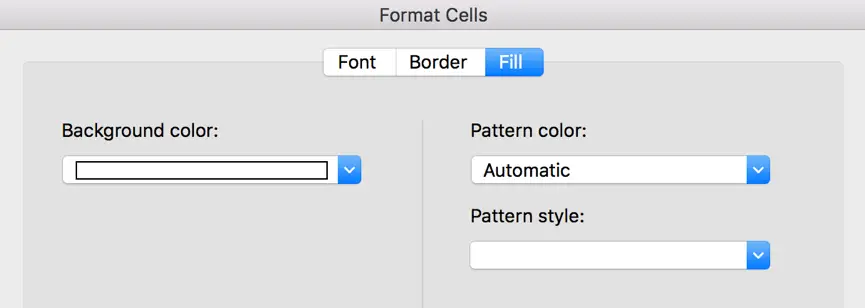
Step 7: Click on Fill, set Background color as No Color, Pattern color as Automatic, then click OK.
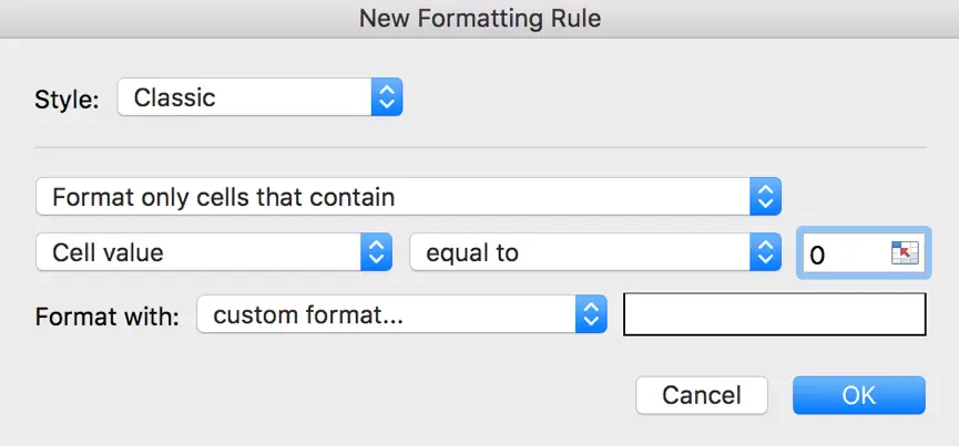
Step 8: After all, on Format Cells screen, click OK to returns to New Formatting Rule screen. Verify that the textbox next to Format with dropdown list is displayed the final format for showing 0 cells. After last several steps, we make 0 values are invisible now.
Now 0 values are invisible in table. Actually 0 values are marked in white color.

Notes:
If you set all background color, border color, pattern color to white, you may get the whole cell covered with white.

3. Hide 0 in Excel by IF Function
If you have a list of number like below, you can use IF function to filter 0 value.
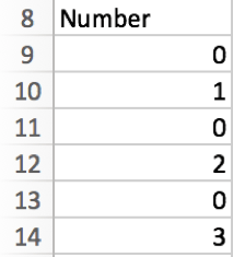
Step 1: In the cell next to A8, enter =IF(A9=0,” “,A9). This formula means if A8=0, then keeps blank in B9, otherwise enter A9 into B9.

Step 2: Drag down B9 filled with formula to other B cells. Now 0 cells are invisible.
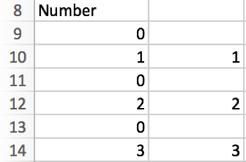
Step 3: Just copy B9-B14 to A9-A14 by paste with Paste Special->Paste Values.
4. Hide 0 in Excel by Uncheck ‘Show a zero in cells that have zero value’ Option
Step 1: Click on File->Options->Advanced to open Excel Options.
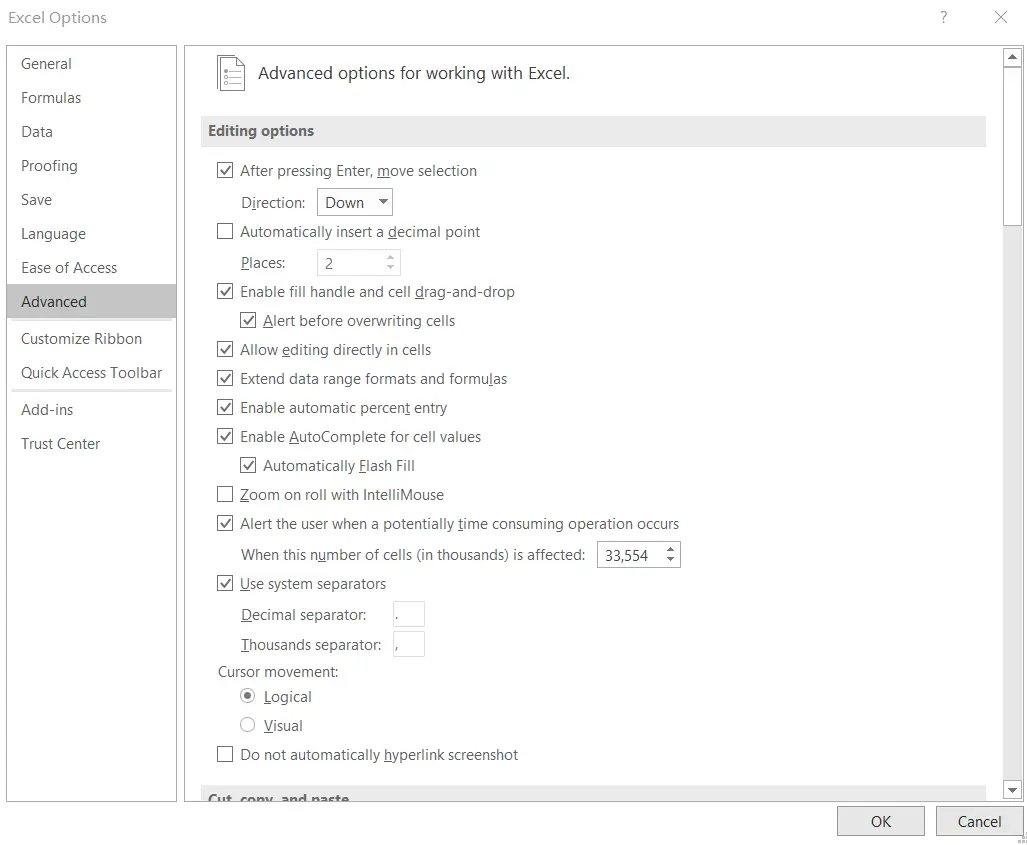
Step 2: Under Display options for this worksheet, you can find there is an option ‘Show a zero in cells that have zero value’. It is checked by default, so normally we can see zero values in our worksheet.

If you uncheck the check box, all zero values are displayed as blank cells in worksheet.
If you check the check box, all zero values are displayed properly.
5. Video: Hide Zero (0) Values
This Excel video tutorial, we’ll guide you through four effective methods to hide zero values in Excel. Whether you prefer using format settings, conditional formatting, the IF function, or adjusting Excel options, we’ve got you covered.
6. Related Functions
- Excel IF function
The Excel IF function perform a logical test to return one value if the condition is TRUE and return another value if the condition is FALSE. The IF function is a build-in function in Microsoft Excel and it is categorized as a Logical Function.The syntax of the IF function is as below:= IF (condition, [true_value], [false_value])….