This post will guide you how to hide zero values in a pivot table in Excel. How do I remove rows with zero values in your pivot table. How to hide rows with zero values in pivot table in Excel 2013/2016.
If you are working with large data sets, you may have noticed that your pivot table displays zero values in empty cells. These zero values can clutter your data and make it harder to read and interpret.
Fortunately, there are a few simple steps you can take to hide zero values in pivot tables. One way is to create a filter field that excludes zero values, or you can format cells to display blank instead of zero. Additionally, you can use the Filter function to remove zero values from your pivot table data.
Table of Contents
1. Hide Zero Values in Pivot Table by Filter Field
If you have created a pivot table based on your data in your current worksheet, and you need to hide the zero values row in your pivot table. You just need to do the following steps to achieve the result.
Step1: select the pivot table in your worksheet, and the PivotTable Fields pane will appear.
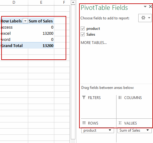
Step2: drag fields which you want to filter or hide zero values from the Choose fields to add to report section to FILTERS section in PivotTable Fields pane.

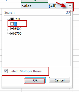
Step3: click the drop down arrow of the field, and check Select Multiple Items, and uncheck 0 value. Click OK button.
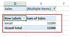
Step4: all zero values in pivot table have been hidden.
2. Hide Zero Values in Pivot Table Using Format Cells Feature
If you want to hide pivot table zero values in Excel, you can use the Format Cells command. This method will not only hide the zero values but also keep the actual values available for calculation purposes. Here are the steps to follow:
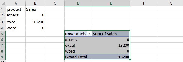
Step1: Select the pivot table cells that contain zero values.
Step2: Right-click and select “Format Cells” from the context menu.

Step3: In the “Format Cells” dialog box, go to the “Number” tab. Under “Category” select “Custom“. In the “Type” field, enter three semicolons 0;-0;;@ .
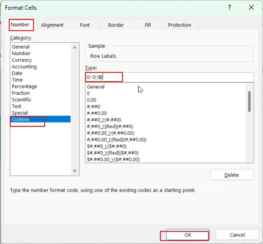
Step4: Click “OK” to apply the custom format.

Now your pivot table will show blank cells instead of zero values, making it easier to read and interpret your data.
3. Hide Zero Values in Pivot Table Using Filter Function
If you want to hide zero value rows in pivot tables in Excel, you can use the Filter function. This method will not delete the rows containing zero values but instead temporarily hide them, making it easier to focus on the relevant data. Here are the steps to follow:
Step1: right click any row content inside the pivot table.
Step2: In the dropdown list, select “Filter” option. And select “Value Filters”.
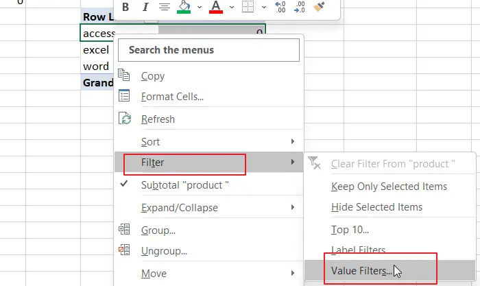
Step3: In the “Value Filter” dialog box, select the type of filter you want to apply, such as “Equals” , “does not equal”, “is greater than,” “is less than”, etc.

For example, if you want to hide all rows that have a value of zero, you can select “does not equal”, and enter “0” as the filter criteria.

Step4: Click “OK” to apply the filter.
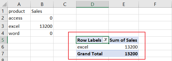
This method will hide all the rows that have zero values in the selected field, and you can quickly unhide them again by checking the box next to “0”.
4. Video: Hide Zero Values in Pivot Table
This video will demonstrate how to hide zero values in pivot tables in Excel using three methods: creating a filter field, formatting cells, and using the Filter function.
Leave a Reply
You must be logged in to post a comment.