This post will guide you how to highlight dates between two dates in your worksheet in Excel. How do I highlight cells between two dates using Conditional Formatting feature in Excel 2013.2016.

Highlight Dates between Two Dates

---

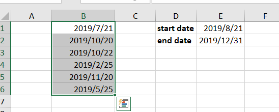
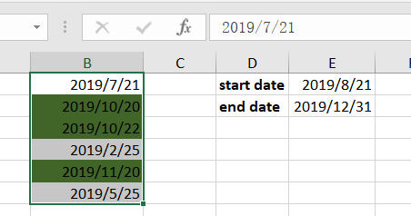
Assuming that you have a list of data in range B1:B6, in which contain date values. and you want to highlight all the dates which are between the range of two dates. such as: you have a start date 2019/8/21 and an end date 2019/12/31, and you want to highlight all the cells in which date is between these two dates. just do the following steps:

Step1: select you range of cells that you want to highlight the date cells.

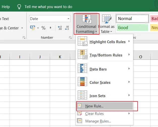
Step2: go to Home tab, and click Conditional Formatting command under Styles group, and select new Rule from the context menu list. and the New Formatting Rule dialog will open.

Step3: click Use a formula to determine which cells to format option in the Select a Rule Type list, and type the following formula into the Format values where this formula is true text box.

=AND($B1>=$E$1,$B1<=$E$1)

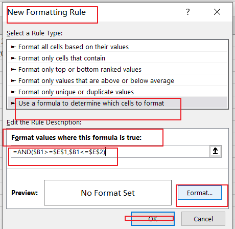
Step4: click Format button in the New Formatting Rule dialog box, and the Format Cell dialog will open.

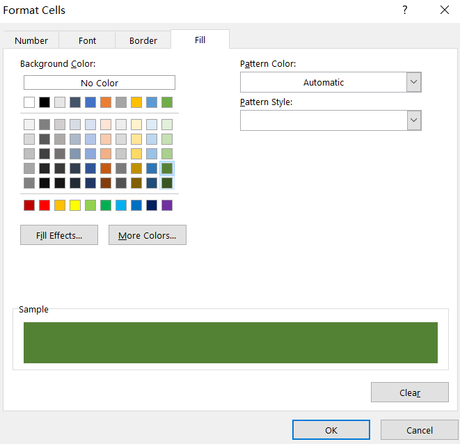
Step5: switch to Fill tab in the Format Cell dialog box, and choose one color as you need. click Ok button back to the New Formatting Rule dialog box.

Step6: click Ok button. You would see that the cells have been highlighted.