Sometimes we may want to highlight every other row or every Nth row in a spreadsheet to make data in different rows looks more clearly. Though we can apply table styles to highlight table rows automatically, we can also highlight rows by excel ‘Conditional Formatting’ function. Actually, ‘Conditional Formatting’ has a powerful capability to highlight cells per some rules, it already contains some rules like ‘Duplicate Values’ in itself, we can also define new rule by ourselves. In this free tutorial, we will introduce you the way to highlight every Nth row through ‘Conditional Formatting->New Rule’ function. Follow steps with screenshots below, we can make sure you can learn it well.
Precondition:
Create a table with several rows. Now we want highlight rows every other row or every Nth row.
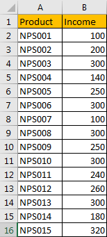
Table of Contents
1. Highlight Every Other Row by Conditional Formatting Function
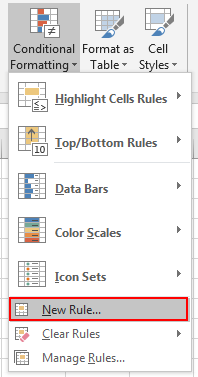
Step1: Select the range to highlight rows, you can ignore the header part. Click Home in ribbon, then click Conditional Formatting in Styles group, select New Rule in menu.
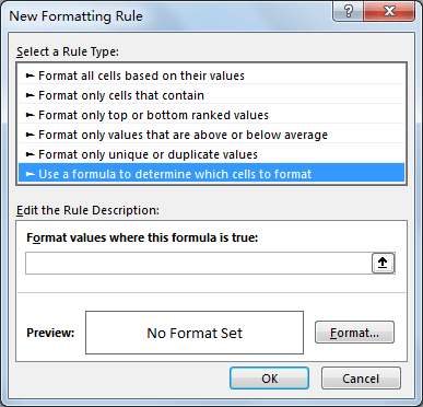
Step2: On New Formatting Rule dialog, select the last rule type: Use a formula to determine which cells to format.
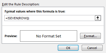
Step3: In Edit the Rule Description section, in Format values where this formula is true textbox enter the formula =ISEVEN(ROW()).
Step4: Click Format button in Preview section. Verify that Format Cells window is displayed.
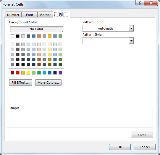
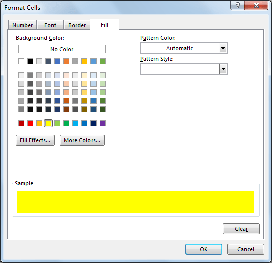
Step5: Click Fill tab, then select a color as background color. For example, select yellow, then click OK.
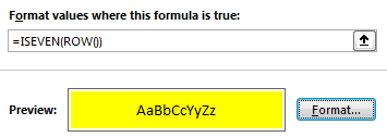
Step6: After above step, we go back to New Formatting Rule window. You can see that in Preview section, cell is filled with yellow. Click OK.
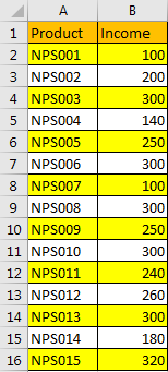
Step7: Check the result. See screenshot below. Rows are highlighted every other row.
2. Highlight Every Nth Row by Conditional Formatting Function
Just repeat above steps, only a little difference in some steps. See simple steps below.
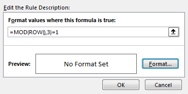
Step1: In above step#3, in Edit the Rule Description section, in Format values where this formula is true textbox enter the formula =MOD(ROW(),3)=1. In this formula, highlight rows every third row.
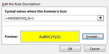
Step2: Select yellow to highlight rows. See preview part.
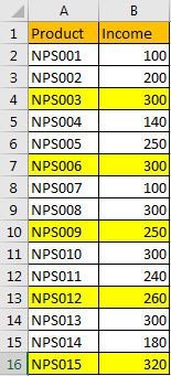
Step3: Check the result, see screenshot below. It works well. If you want the header part is also included in counting, you can update the formula as =MOD(ROW(),3)=0.
3. video: Highlight Every Other Row or Every Nth Row
This Excel video tutorial where we’ll enhance your spreadsheet readability by exploring two conditional formatting functions. First, we’ll learn how to highlight every other row, followed by a more advanced method to highlight every Nth row.
4. Related Functions
- Excel ROW function
The Excel ROW function returns the row number of a cell reference.The ROW function is a build-in function in Microsoft Excel and it is categorized as a Lookup and Reference Function.The syntax of the ROW function is as below:= ROW ([reference])…. - Excel MOD function
he Excel MOD function returns the remainder of two numbers after division. So you can use the MOD function to get the remainder after a number is divided by a divisor in Excel. The syntax of the MOD function is as below:=MOD (number, divisor)….