This post will guide you how to highlight every other row in Excel. How do I shade every other row with conditional formatting in Excel.

• Highlight Every Other Row
• Video: Highlight Every Other Row

Highlight Every Other Row

---

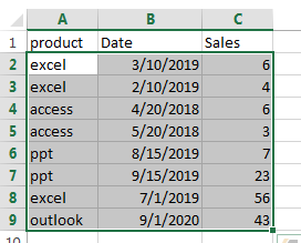
Assuming that you have a list of data in range A1:C9, and you want to highlight every second product name in your data. And you can easily achieve the result using conditional formatting feature. The below are steps to highlight every second row in Excel:

#1 select the range of cell A2:C9 which you want to highlight every second row.

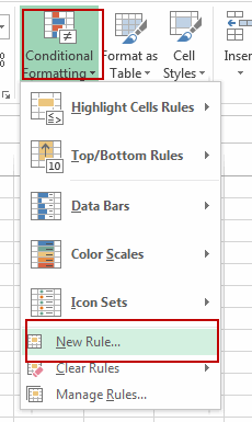
#2 go to HOME tab, click the Conditional Formatting command under Styles group. Then select New Rules… from the drop-down menu list.

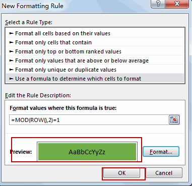
3# the New Formatting Rule window will appear.

4# select the Use a formula to determine which cells to format option under Select a Rule Type: box, and then enter the following formula in the Format values where this formula is true: box:

=MOD(ROW(),2)=1

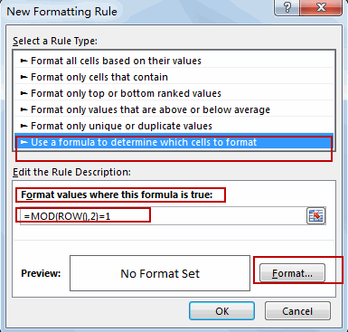
Note: The MOD function returns the remainder when the row number is divided by 2. And it will check each cell if it meets the criteria. And it will check Cell A2 firstly, and the row function in Cell A2 would return 2, and the MOD(2,2) formula returns 0, which does not meet our criteria. And then it will move on the other cell to check it based on the formula. If it returns 1, then it matches the criteria. It highlights the entire row.

5# click the Format… button, then the Format Cells window will appear.

6# in the “Format Cells” window, switch to the Fill tab, choose the background color, and then click OK button. You can also switch to other tabs to tweak the settings as you want.

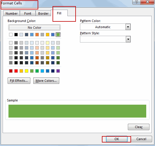
7# back in the New Formatting Rule window, you can see a preview of your rows background color. Then click OK button.

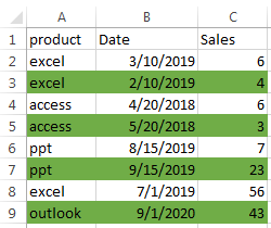
You will see that every second row have been highlighted with the background color as you set.

Video: Highlight Every Other Row

Related Functions

---

• Excel ROW function
  The Excel ROW function returns the row number of a cell reference.The ROW function is a build-in function in Microsoft Excel and it is categorized as a Lookup and Reference Function.The syntax of the ROW function is as below:= ROW ([reference])….
• Excel MOD function
  he Excel MOD function returns the remainder of two numbers after division. So you can use the MOD function to get the remainder after a number is divided by a divisor in Excel. The syntax of the MOD function is as below:=MOD (number, divisor)….